
QForte: A quantum computer simulator and algorithms library for molecular simulation
Background
Classical simulation of molecules and materials via solution of the Schröodinger equation is largely prevented by exponentially scaling memory requirements.8 Quantum computational simulation offers a way to circumvent the storage bottleneck. An \(n\) qubit register is capable of storing a state in a Hilbert space of dimension \(2^n\), and operations can be applied to the entire state in constant time.2 In tandem with the development of physical quantum hardware, it is imperative that open-source implementations of emerging quantum algorithms be made available to better facilitate future development as well as cross-comparison of methods. QForte is aimed at addressing such a need.
What is QForte?
QForte is an open-source package with two main components. First, it is an open-source
quantum computer simulator written in C++ and exposed in Python via pybind11.
They key elements of a simulated quantum computation are building a quantum register, applying circuits
to the register, and measuring expectaion values.
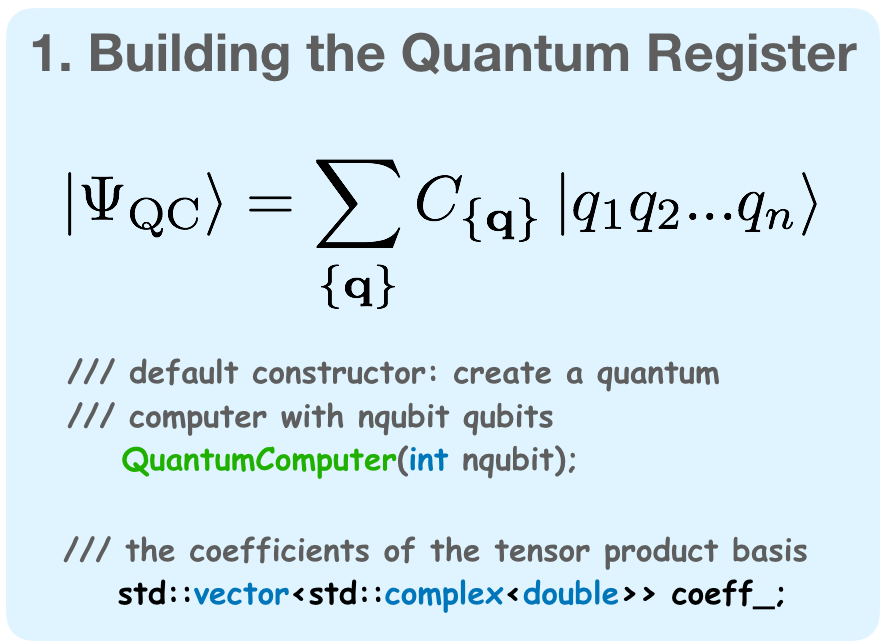
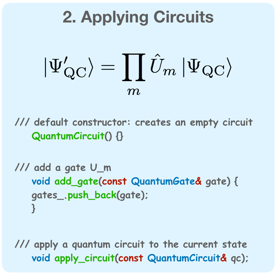
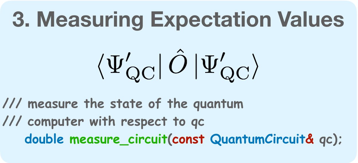
Figure 1: The three aspects of a simulated quantum computation.
Second, it is a library of quantum computational algorithms aimed at simulating
molecular systems. This combination allows the user to calculate molecular properties
(such as the energy) using a specified quantum algorithm with just a few lines of code,
similar to what would be required to run a calculation using a classical quantum chemistry
package. It utilizes simple interfaces to Psi4 and OpenFermion to generate molecular integrals.
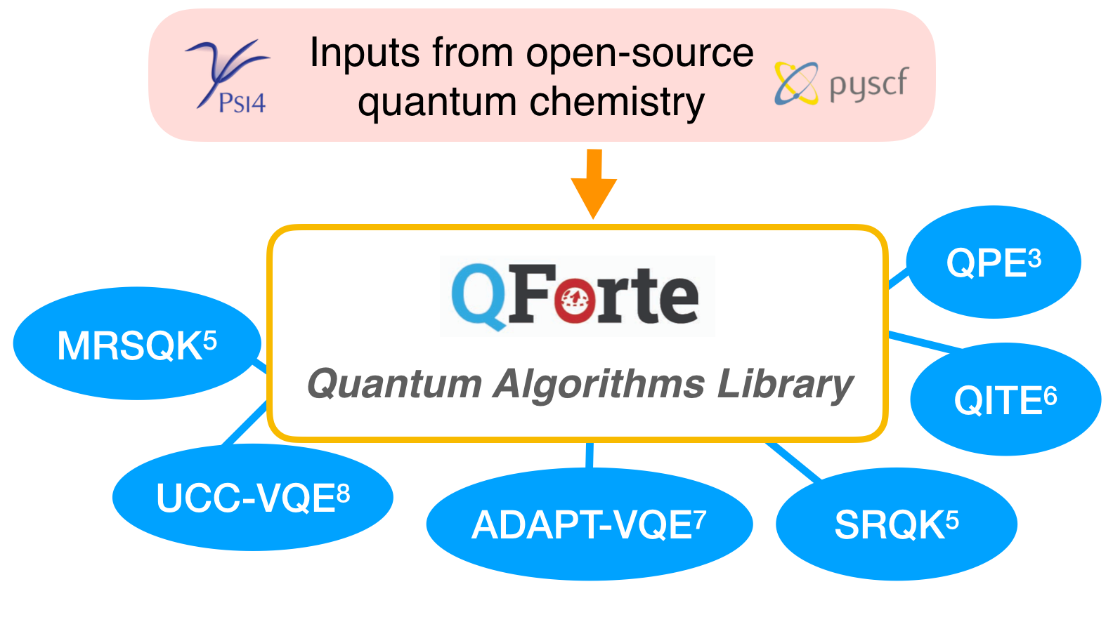 Figure 2: QForte algorithms library.
Why is QForte useful?
Recent advances in quantum computational hardware has sparked a massive influx of exciting new quantum algorithms suitable for molecular simulation. However, the vast majority of algorithms are published without performance comparisons to existing methods, primarily due to lack of software availability. Moreover, many metrics are required to adequately compare the utility of quantum algorithms. For example, the number of multi-qubit operations, the number of operator measurements, the number of variational classical parameters, and the error in the property of interest are all important considerations.
Compare with existing algorithms
QForte offers an easy-to-use option for algorithm comparison, capable of reporting the above values in a unified fashion for a variety of state-of-the-art quantum algorithms. The list of presently available algorithms includes: quantum phase estimation (QPE),3 single reference quantum Krylov (SRQK),4,5 multireference selected quantum Krylov (MRSQK),5 quantum imaginary time evolution (QITE),6 the adaptive derivative assembled pseudo Trotterized variational quantum eigensolver (ADAPT-VQE),7 and unitary coupled cluster singles and doubles VQE (UCCSD-VQE).8
Development toolbox for new algorithms
QForte also serves as a powerful tool for the development of new algorithms using abstract bass classes to ensure uniformity. It contains fast C++ implementations of the Jordan-Wigner transform, circuit application, Trotterization, state overlap, and operator measurement. These tools allow for rapid development of VQE and QK ansatz or even entirely new classes of algorithms.
Example usage
Build the Bell state on a quantum computer.
1
2
3
4
5
6
7
8
9
10
11
12
13
14
15
16
17
18

import qforte as qf

# define the number of qubits
nqbits = 2

# construct a quantum computer
computer = qf.QuantumComputer(nqbits)

# construct Hadamard and CNOT gates
H_0 = qf.make_gate('H',0,0)
cX1_0 = qf.make_gate('cX',1,0)

# apply the gates
computer.apply_gate(H_0)
computer.apply_gate(cX1_0)

# print the state of the quantum register
print(computer)
Output:
QuantumComputer(
  (0.707107 +0.000000 i) |00>
  (0.000000 +0.000000 i) |10>
  (0.000000 +0.000000 i) |01>
  (0.707107 +0.000000 i) |11>
 )
Run quantum phase estimation on H2.
1
2
3
4
5
6
7
8
9
10
11
12
13
14
15
16
17
18
19
20
21
22
23

# import qforte
import qforte
from qforte.qpea.qpe import QPE
from qforte.system import system_factory

# define geometries and reference list
H2geom = [('H', (0., 0., 0.)), ('H', (0., 0., 1.50))]
H2ref = [1,1,0,0]

# run classical SCF
adapter = system_factory(mol_geometry=H2geom)
adapter.run()
H2mol = adapter.get_molecule()

# constrct and run QPE algorithm
alg = QPE(H2mol, H2ref, trotter_number=2)
alg.run(t = 0.4,
        nruns = 100,
        success_prob = 0.5,
        num_precise_bits = 8)

# get desired properties
Egs = alg.get_gs_energy()
Output:
Using standard openfermion hamiltonian ordering!

-----------------------------------------------------
       Quantum Phase Estimation Algorithm
-----------------------------------------------------


                 ==> QPE options <==
-----------------------------------------------------------
Trial reference state:                    |1100>
Trial state preparation method:           reference
Trotter order (rho):                      1
Trotter number (m):                       2
Use fast version of algorithm:            True
Measurement varience thresh:              NA
Target success probability:               0.5
Number of precise bits for phase:         8
Number of time steps:                     10
Evolution time (t):                       0.4
Number of QPE algorithm executions:       100


           ==> QPE readout averages <==
------------------------------------------------
  bit  0 :  0.0
  bit  1 :  0.0
  bit  2 :  0.0
  bit  3 :  0.86
  bit  4 :  0.0
  bit  5 :  0.14
  bit  6 :  0.0
  bit  7 :  0.14
  bit  8 :  0.01
  bit  9 :  0.85

  Final bit readout:  [0, 0, 0, 1, 0, 0, 0, 0, 0, 1]


                        ==> QPE summary <==
---------------------------------------------------------------
Final QPE Energy:                         -0.9970875121
Mode QPE Energy:                          -0.9970875121
Final QPE phase:                           0.0634765625
Mode QPE phase:                            0.0634765625
Run ADAPT-VQE on Be.
1
2
3
4
5
6
7
8
9
10
11
12
13
14
15
16
17
18
19
20
21
22
23

# import qforte
import qforte
from qforte.ucc.adaptvqe import ADAPTVQE
from qforte.system import system_factory

# define geometries and reference list
Be_geom = [('Be', (0., 0., 0.))]
Be_ref = [1,1,1,1,0,0,0,0,0,0]

# run classical SCF
adapter = system_factory(mol_geometry=Be_geom)
adapter.run()
Be_mol = adapter.get_molecule()

# constrct and run ADAPT-VQE
alg = ADAPTVQE(Be_mol, Be_ref, trotter_number=1)
alg.run(adapt_maxiter=5,
        avqe_thresh=0.1,
        op_select_type='gradient',
        use_analytic_grad=True)

# get desired properties
Egs = alg.get_gs_energy()
Output:
Using standard openfermion hamiltonian ordering!

-----------------------------------------------------
  Adaptive Derivative-Assembled Pseudo-Trotter VQE
-----------------------------------------------------


               ==> ADAPT-VQE options <==
---------------------------------------------------------
Trial reference state:                    |1111000000>
Trial state preparation method:           reference
Trotter order (rho):                      1
Trotter number (m):                       1
Use fast version of algorithm:            True
Measurement varience thresh:              NA
Optimization algorithm:                   BFGS
Optimization maxiter:                     200
Optimizer grad-norm threshold (theta):    1.00e-05
Use analytic gradient:                    True
Operator pool type:                       SD
ADAPT-VQE grad-norm threshold (eps):      1.00e-01
ADAPT-VQE maxiter:                        5


==> Building comutator pool for gradient measurement.
==> Comutator pool construction complete.


 -----> ADAPT-VQE iteration  0  <-----

==> Measring gradients from pool:
 Norm of <[H,Am]> =   0.22748321
 Max  of <[H,Am]> =  -0.12276644
  Adding operator m = 21

toperators included from pool:
 [21]
tamplitudes for tops:
 [0.0]

--> Begin opt with analytic graditent:
  Initial guess energy:  -14.351880476202027
  minimization successful.
  min Energy:  -14.37279090388743


 -----> ADAPT-VQE iteration  1  <-----

==> Measring gradients from pool:
 Norm of <[H,Am]> =   0.16804755
 Max  of <[H,Am]> =  -0.10822623
  Adding operator m = 24

toperators included from pool:
 [21, 24]
tamplitudes for tops:
 [0.33428557457187374, 0.0]

--> Begin opt with analytic graditent:
  Initial guess energy:  -14.37279090388743
  minimization successful.
  min Energy:  -14.389439069292933


 -----> ADAPT-VQE iteration  2  <-----

==> Measring gradients from pool:
 Norm of <[H,Am]> =   0.11575674
 Max  of <[H,Am]> =  -0.09869260
  Adding operator m = 26

toperators included from pool:
 [21, 24, 26]
tamplitudes for tops:
 [0.2946784148978646, 0.3012771224143545, 0.0]

--> Begin opt with analytic graditent:
  Initial guess energy:  -14.389439069292933
  minimization successful.
  min Energy:  -14.403328602115806


 -----> ADAPT-VQE iteration  3  <-----

==> Measring gradients from pool:
 Norm of <[H,Am]> =   0.05300504
 Max  of <[H,Am]> =   0.02825606

  ADAPT-VQE converged!


                ==> ADAPT-VQE summary <==
-----------------------------------------------------------
Final ADAPT-VQE Energy:                      -14.403328602
Number of operators in pool:                  27
Final number of amplitudes in ansatz:         3
Total number of Hamiltonian measurements:     21
Total number of comutator measurements:       127
References
-
Laughlin, Robert B., and David Pines. “From the cover: The theory of everything.” Proceedings of the national academy of sciences of the United States of America 97.1 (2000): 28.
-
Cao, Yudong, et al. “Quantum chemistry in the age of quantum computing.” Chemical reviews 119.19 (2019): 10856-10915.
-
Abrams, Daniel S., and Seth Lloyd. “Quantum algorithm providing exponential speed increase for finding eigenvalues and eigenvectors.” Physical Review Letters 83.24 (1999): 5162.
-
Parrish, Robert M., and Peter L. McMahon. “Quantum filter diagonalization: Quantum eigendecomposition without full quantum phase estimation.” arXiv preprint arXiv:1909.08925 (2019).
-
Stair, Nicholas H., Renke Huang, and Francesco A. Evangelista. “A multireference quantum krylov algorithm for strongly correlated electrons.” Journal of Chemical Theory and Computation 16.4 (2020): 2236-2245.
-
Motta, Mario, et al. “Determining eigenstates and thermal states on a quantum computer using quantum imaginary time evolution.” Nature Physics 16.2 (2020): 205-210.
-
Grimsley, Harper R., et al. “An adaptive variational algorithm for exact molecular simulations on a quantum computer.” Nature communications 10.1 (2019): 1-9.
-
Peruzzo, Alberto, et al. “A variational eigenvalue solver on a photonic quantum processor.” Nature communications 5 (2014): 4213.
Acknowledgements
Nicholas H. Stair was supported by a fellowship from The Molecular Sciences Software Institute under NSF grant OAC-1547580