PDFT - An accessible density embedding code

Introduction

• Density embedding methods avoid the exponential scaling that hinders users from using accurate quantum chemistry in large and complex systems. Partition Density Functional Theory (PDFT)[1-4], makes use of functionals of non-interacting fragments, so that the energy of the entire system and any other electronic properties is given by functionals of the set of the less computationally demanding fragment densities. In PDFT we minimize \(E_f \equiv \sum_i E_i[ n_i ]\) while satisfying the density constraint \(\sum_i n_i(\mathbf{r}) = n_m(\mathbf{r})\).

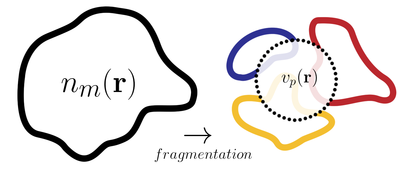Figure 1: The unique local potential \(v_p(\mathbf{r})\) ensures that the fragment densities sum up to the total correct density \(n(\mathbf{r})\)

• The caveat is that an extra component–that accounts for the inter-fragment interaction–is missing: The partition potential. This extra component modifies the external potential of each fragment just slightly so that the sum of all the fragment densities matches the molecular density. Finding out what the partition potential is for a given set of fragments, whether using an “exact” or approximated potential, is our code’s goal.

Calculations with PDFT

• PDFT is written in the interpreted language Python, and it strives to be readable, reliable and reusable. We do this is by enforcing the programming best practices that are being set by the greater community of the computational molecular sciences.

• PDFT makes use of the PSIAPI[5] and thus is written similarly to Psi4Numpy[6]. The most basic calculation in PDFT is a self-consistent calculation. The SCF solves the Kohn-Sham equations by diagonalizing the DFT Fock Matrix:

\[F^{DFT}_{\mu \nu} = H_{\mu \nu} + 2J[D]_{\mu \nu} - \zeta K[D]_{\mu \nu} + V^{xc}_{\mu \nu}\]

Basic Calculation

Making a DFT calculation in PDFT is extremely easy, and users of Psi4Numpy will find it extremely familiar. Given an exchange-correlation approximation available in Libxc[7], one can calculate the energy of a molecule. As an example, the energy for a Hydrogen atom with the Local Density Approximation (LDA) in the Universal Gaussian Basis set (UGBS) is computed as:

import psi4
import pdft

psi4.set_options({“reference”:”uhf”})

#Geometry Definition
H_geo = psi4.geometry(“””
0 2
H””)

#Define pdft object and run scf cycle
H = pdft.UMolecule(H_geometry, “ugbs”, “svwn”)
h.scf()

Notice that PDFT uses the molecule class of Psi4, but it is then used to define an instance of the class UMolecule. PDFT contains two main classes, RMolecule and UMolecule. Both are inherited from a parent class Molecule, that allows modifications to be directly reflected on each child, making additions, troubleshooting and debugging a breeze.

Getting information on the grid

The components of the Fock-Matrix and other results from the scf calculation are expressed in the atomic orbital (ao) basis. Several steps are required to be able to visualize any of those quantities on the grid. PDFT has a wide variety of elements available on the grid directly as attributes. Information on the grid can quickly be requested by adding some arguments to the scf method:

h.scf(get_ingredients=True, get_orbitals=True)

The first option get_ingredients stores components relevant to the development of Density Functional Approximations (DFA), such as the density and its derivatives, kinetic energy density and contributions to the Kohn-Sham potential. Whereas the latter option get_orbitals stores each of the molecular orbitals both on the atomic orbital basis and on the grid.

To highlight the effortless visualization of quantities relevant to developers in the DFT community, Figure 2 and Figure 3 show two examples of the aforementioned quantities on the grid that are commonly explored in the literature[8,9].

Consider the ubiquitous self-Interaction error: An exchange-correlation potential from a DFA will typically not be able to fully cancel out the Hartree potential for a one-electron system, generating a spurious behavior where an electron will interact with itself. Consider the calculation we performed for Hydrogen using LDA, after running the scf cycle we can visualize the potentials by simply typing:

vha = h.potential["vha"]
vxc = h.potential["vxc"]
sie = vha + vxc

h.axis_plot_r([vha, vxc, sie], labels=["V_Hartree", "v_xc", "v_Hxc"])

The method axis_plot_r simply looks at information in 1D, in this case the axis that runs through the atom. In the future, this function will allow the user to select any line in space, or any plane in space. If ran within a Jupyter Notebook, the previous line will generate a plot as seen in Figure 2. Nevertheless one can export the data on the grid to be used elsewhere.

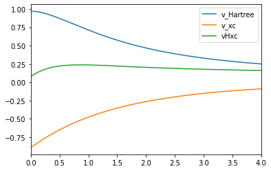
Figure 2: Self-interaction error of the LDA for the Hydrogen atoms.

Besides from potentials, the electron density and its derivatives are also available. For example, lets visualize some ingredients used in the development of generalized gradient approximations. Consider a HF/UGBS calculation of the Kr atom.

#Basic calculation:
Kr_geometry = psi4.geometry("""
0 1
Kr 0.0 0.0 0.0
units bohr
symmetry c1
""")

Kr = pdft.UMolecule(Kr_geometry, "ugbs", "hf")
Kr.scf(get_matrices=True, get_ingredients=True, get_orbitals=True)

r = []
for i_block in range(Kr.nblocks):
    r.append((Kr.grid["x"][i_block]**2 + Kr.grid["y"][i_block]**2 + Kr.grid["z"][i_block]**2)**(1/2))
r = np.array(r)
    
density = Kr.ingredients["density"]["da"] + Kr.ingredients["density"]["db"]
    
#Density
n =(4 * np.pi * r**2) * density

#Gradient
s =  (Kr.ingredients["gradient"]["da_x"] + Kr.ingredients["gradient"]["db_x"])**2
s += (Kr.ingredients["gradient"]["da_y"] + Kr.ingredients["gradient"]["db_y"])**2
s += (Kr.ingredients["gradient"]["da_z"] + Kr.ingredients["gradient"]["db_z"])**2
for i_block in range(Kr.nblocks):
    s[i_block] = np.sqrt(s[i_block])
s /= density**(4/3)

#Laplacian
q = Kr.ingredients["laplacian"]["la_x"] + Kr.ingredients["laplacian"]["lb_x"]
q += Kr.ingredients["laplacian"]["la_z"] + Kr.ingredients["laplacian"]["lb_y"]
q += Kr.ingredients["laplacian"]["la_y"] + Kr.ingredients["laplacian"]["lb_z"]
q /= density**(5/3)

After running the scf calculation, one can build the ingredients involving the density, gradient and laplacian. They can be individually seen in Figure 3.

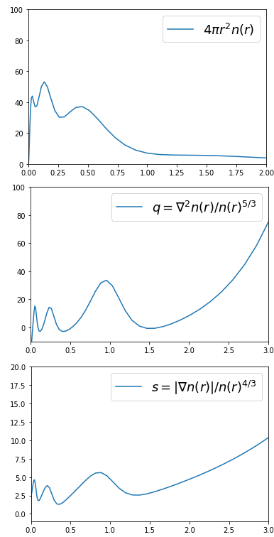
Figure 3: Dimensionless ingredients of GGA’s for a Kr atom.

Advanced methods in PDFT

Having an scf cycle completely written in Python allows it to be quickly modified to suit the developers needs. For example, in embedding methods, we are required to add an external potential to each of the fragments. Assuming one has a partition potential \(v_p(r)\) expressed in the ao basis, one can simply run the following to solve self-consistently:

h.scf(vp=potential_mn)

Density-to-Potential inversions.

The previous feature is required for the development of inversion methods. Where a potential–such as the embedding potential–can be obtained “exactly” (for a given DFA and a basis set) by using a density-to-potential algorithm. Such an algorithm is exemplified in Figure 4.

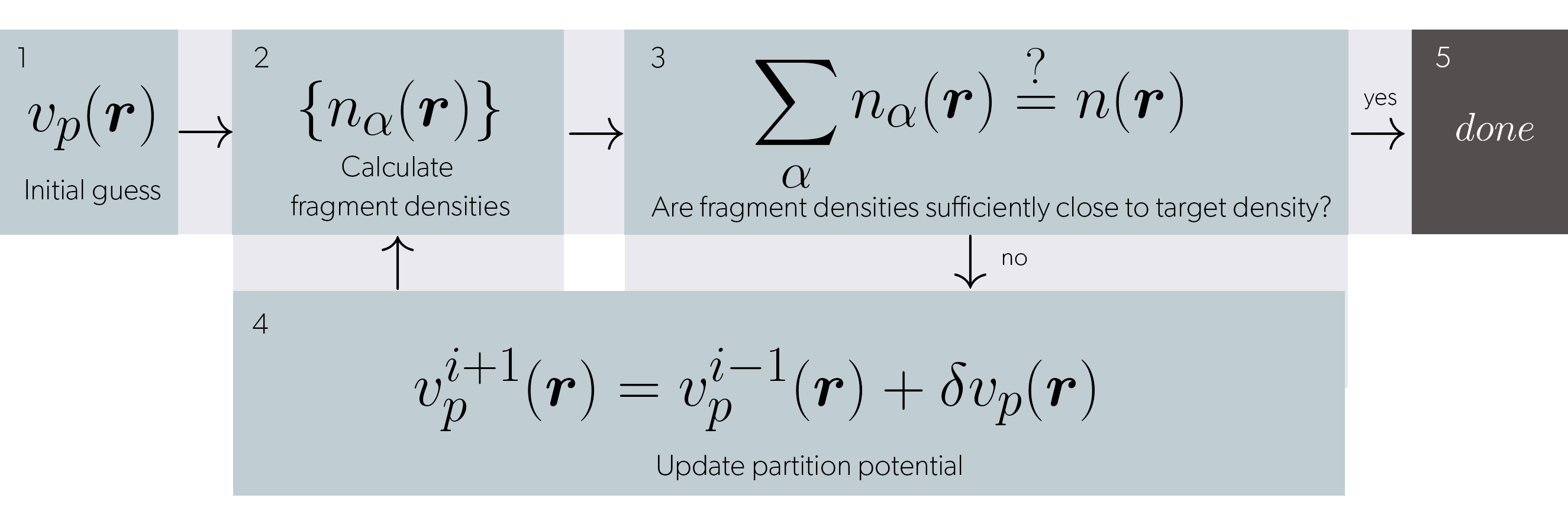
Figure 4: Algorithm for the generation of an embedding potential given a set of fragments and a target density.

The previous algorithm is implemented in the Inversion class within PDFT. Such a class takes as arguments fragments and target systems in the same ao basis and builds the relevant information for inversion. (e.g. density differences and non-additive quantities). One can select many different methods to compute \(\delta v_p(r)\) of step 4. It is known that these methods can be very finicky and dependant on parameters, initial guess and choice of basis set. Although basic algorithms such as density difference and ZMP[10] are already implemented, we are working on making other methods available such as Wu-Yang[11] and Ou-Carter[12]. We are striving for these methods to be reliable and require minimum input from the user. With orbitals, and other ingredients available at ease, we are confident that our code will provide a quick and easy way to implementing and benchmarking new inversion methods.

Future of PDFT

To be (approximated) or not to be: That is the question

Although inversions required for finding the exact embedding potential, in practice one could approximate the non-additive kinetic energy functional (NAKE) \(T_s^{nad}[{ n_i }] = T_s[n_m] - \sum_i T_s[n_i]\). PDFT will have an abstract class for the NAKE functional with a consistent set of attributes that will provide a blueprint for new proposed functionals from the broader research community.

Fractional Charges

By generalizing PDFT to fragments with non-integer occupations, it is possible to remove the static-correlation and delocalization errors. This is done by defining an ensemble of two systems, each with an integer number of electrons \(E_{\omega} = \omega E[N+1] + (1 - \omega)E[N]\), where the argument in each term refers to a density that integrates to N and N+1 electron. By doing so it will be possible to obtain qualitatively correct results for system in different molecular environments such as charge transfer. This capability will soon be implemented in our Molecule class.

References

1. Jonathan Nafziger and Adam Wasserman. Density-based partitioning methods for ground-state molecular calculations. The Journal of Physical Chemistry A, 118(36): 7623–7639, 2014.
2. Peter Elliott, Kieron Burke, Morrel H. Cohen, and Adam Wasserman. Partition densityfunctional theory. Physical Review A, 82(2):024501, 2010.
3. Martin A. Mosquera and Adam Wasserman. Partition density functional theory and its extension to the spin-polarized case. Molecular Physics, 111(4):505–515, 2013.
4. Victor H. Chavez and Adam Wasserman. Towards a density functional theory of molecular fragments. what is the shape of atoms in molecules? Revista de la Academia Colombiana de Ciencias Exactas, Fisicas y Naturales, 44(170):269–279, 2020
5. Smith, D. G., Burns, L. A., Simmonett, A. C., Parrish, R. M., Schieber, M. C., Galvelis, R., … & James, A. M. (2020). PSI4 1.4: Open-source software for high-throughput quantum chemistry. The Journal of Chemical Physics, 152(18), 184108.
6. Smith, D. G., Burns, L. A., Sirianni, D. A., Nascimento, D. R., Kumar, A., James, A. M., … & Berquist, E. J. (2018). Psi4NumPy: An interactive quantum chemistry programming environment for reference implementations and rapid development. Journal of chemical theory and computation, 14(7), 3504-3511.
7. Lehtola, S., Steigemann, C., Oliveira, M. J., & Marques, M. A. (2018). Recent developments in libxc—A comprehensive library of functionals for density functional theory. SoftwareX, 7, 1-5.
8. Gaiduk, A. P., Mizzi, D., & Staroverov, V. N. (2012). Self-interaction correction scheme for approximate Kohn-Sham potentials. Physical Review A, 86(5), 052518.
9. Gaiduk, A. P., & Staroverov, V. N. (2011). Construction of integrable model Kohn-Sham potentials by analysis of the structure of functional derivatives. Physical Review A, 83(1), 012509.
10. Qingsheng Zhao, Robert C. Morrison, and Robert G. Parr. From electron densities to Kohn-Sham kinetic energies, orbital energies, exchange-correlation potentials, and exchange-correlation energies. Physical Review A, 50(3):2138, 1994.
11. Qin Wu and Weitao Yang. A direct optimization method for calculating density functionals and exchange–correlation potentials from electron densities. The Journal of Chemical Physics, 118(6):2498–2509, 2003.
12. Ou, Q., & Carter, E. A. (2018). Potential Functional Embedding Theory with an Improved Kohn–Sham Inversion Algorithm. Journal of Chemical Theory and Computation, 14(11), 5680-5689.

Acknowledgements

Victor H. Chavez was supported by a fellowship from The Molecular Sciences Software Institute under NSF grant OAC-1547580. Victor H. Chavez thanks Yuming Shi and Yan Oueis for helpful conversations.