Latent space representation learning as an auxiliary task for training neural network potentials

Introduction

Molecular properties can be obtained through a description of the electronic structure of any molecular system, which can be derived from high-level ab initio quantum mechanics (QM) by solving the Schrodinger equation. However, finding the exact solution to the many-body Schrodinger equation is NP-hard, or more specifically, QMA-hard (1), which means it is likely to be impossible to find the solution in polynomial time, even with quantum computers.

Various numerical approximations and computational techniques are proposed to accommodate the substantial cost of these calculations to generate results in a reasonable time-frame. These techniques have become integral for the early stages of drug discovery in cases where the selected methods need to match the fast pace of drug design settings in a cost-effective manner. A method that performs as fast as classical force fields and as accurate as high-level QM models is in high demand.

ANI (2) is a deep neural network potential trained to high precision QM methods to generate a transferable and extensible model that can predict molecular energies and forces. ANI potentials, in a suitable framework, can be applied to run dynamical simulations to quickly and accurately study the time evolution of biological systems.

ANI Network Architecture

ANI uses atomic environment vectors (AEV)—a fixed-size representation of the local chemical environment, to predict the contribution of each atom to the total energy of the system. AEV symmetry functions are invariant under translation and rotation and were introduced by Behler and Parrinello (3). These functionals are a combination of two-body (radial) and three-body (angular) terms which encode information regarding the local environment of the atom up to a specific cutoff.

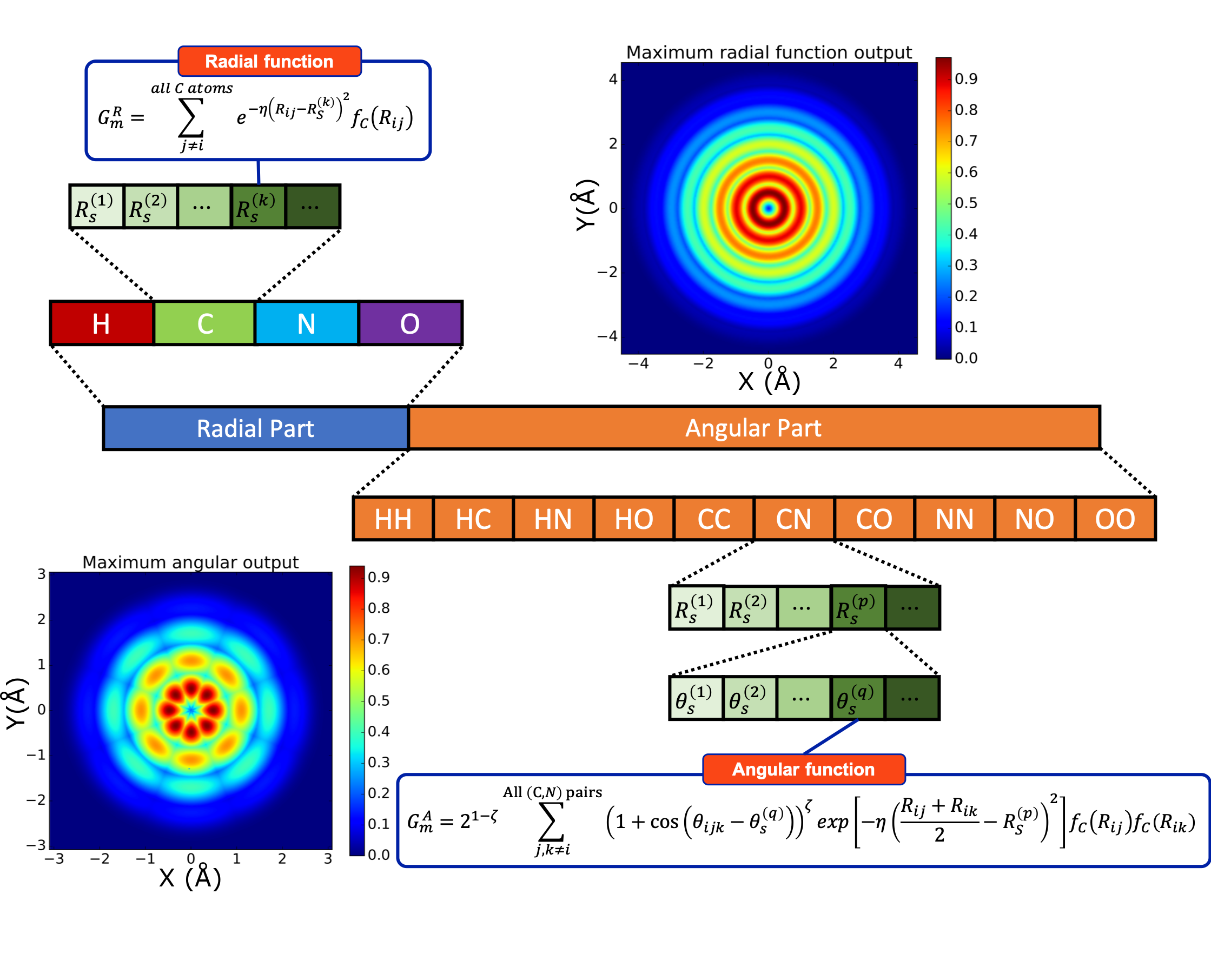
Figure 1: The Structure of the ANI AEVs. The sum of \(j\) and \(k\) is on all neighbor atoms of selected species/pair of species. \(R_s\) and \(\theta_s\) are hyper-parameters called radial/angular shifts. The \(f_C\) is called cutoff cosine function, defined as \(f_C(R)=\frac{1}{2}\left[\cos\left(\frac{\pi R}{R_C}\right) + 1\right]\) for \(R\leq R_C\) and \(0\) otherwise, where \(R_C\) is called cutoff radius, a hyperparameter that defines how far we should reach when investigating chemical environments. Image and caption taken from reference 4.

ANI Network architecture consists of a series of atomic feed-forward networks that input the coordinates \(q\) and atomic numbers \(Z\). Atomic AEVs are calculated and passed to the corresponding atomic network, which predicts their contribution to the molecular energy.

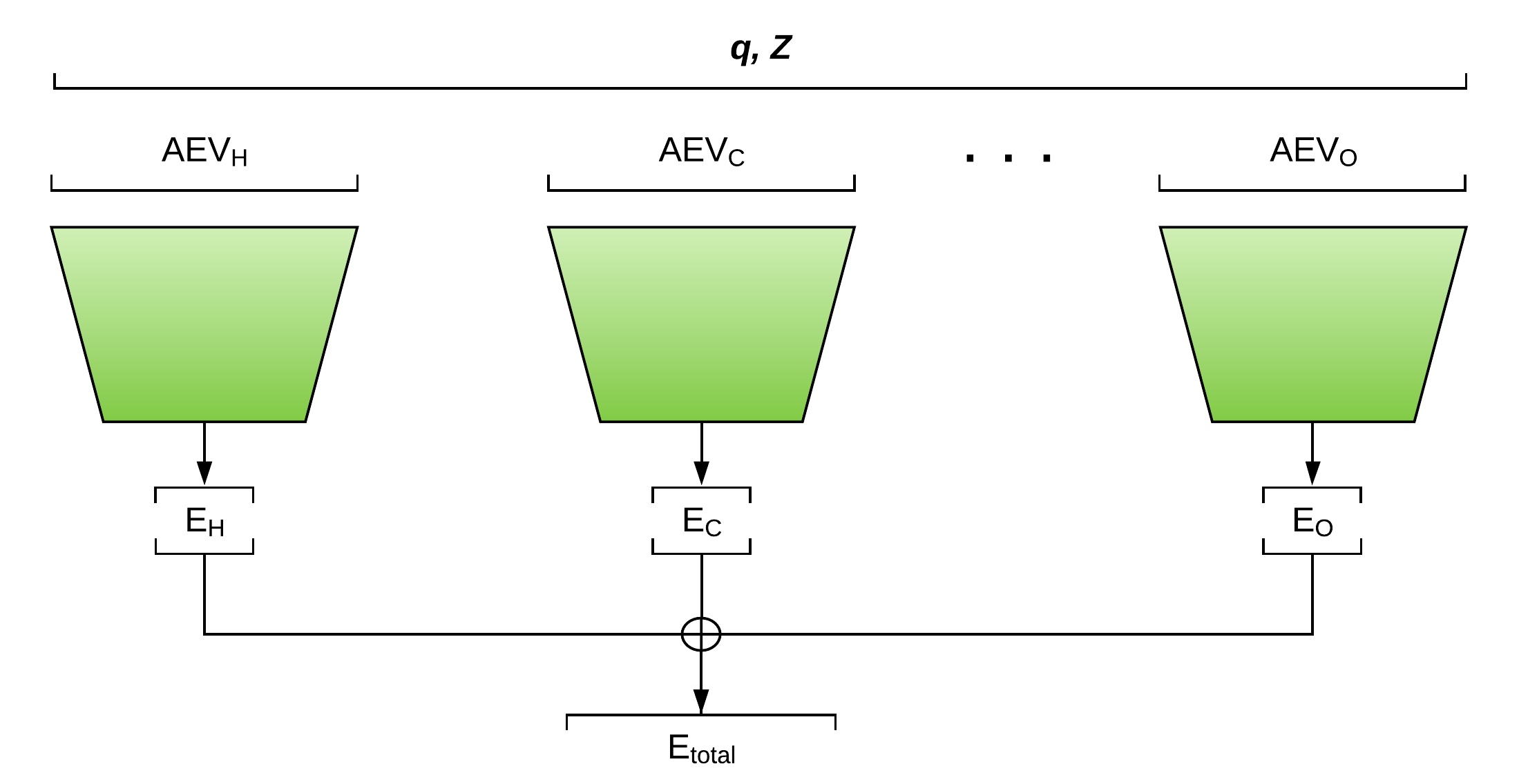Figure 2: ANI Neural Network Architecture

TorchANI

TorchANI (4) is an open-source PyTorch based implementation of ANI that provides a scalable framework for training and inference of deep learning models that benefits from an optimized chemical environment predictor.

TorchANI currently includes tools for inference and training of popular ANI-1x(5), ANI-1ccx(6), and ANI-2x(7) potentials. Predicting ANI energies and forces for a given molecule (e.g., methane) is easily achieved through the following few lines of code using TorchANI:

import torch
import torchani

model = torchani.models.ANI2x(periodic_table_index=True)
coordinates = torch.tensor([[[0.03,  0.006,  0.01],
                             [-0.8,  0.4, -0.3],
                             [-0.7, -0.8,  0.2],
                             [0.5,   0.5,  0.8],
                             [0.7,  -0.2, -0.9]]],
                           requires_grad=True)
# atomic numbers for C, H, H, H, H
species = torch.tensor([[6, 1, 1, 1, 1]])
_, energy = model((species, coordinates))
force = -torch.autograd.grad(energy.sum(), coordinates)[0]

print('Energy:', energy.item())
print('Force:', force.squeeze())

Moreover, PyTorch autograd engine provides access to all the gradients in the computational graph. In the above example, the forces were predicted using the gradients of output molecular energy with respect to the input coordinates. Having access to the gradients one can compute a list of other physical properties such as hessian, vibrational frequencies, stress tensor, and infrared intensities.

TorchANI is interfaced with various computational chemistry packages, including the MolSSI QCArchive software stack, that uses ANI models for data generation via QCEngine.

TorchANI has a design emphasis on being lightweight, user-friendly, cross-platform, and easy to read/modify for fast prototyping of neural network architectures for molecular/atomic properties prediction. In the following sections, an example of such implementation—an AutoEncoder is explained.

Multi-Task Learning

Training a neural network to learn a set of tasks that could benefit from having shared low-level features, provides a considerable amount of knowledge to augment the otherwise relatively small examples for single-task training, a process known as implicit data augmentation.

Multi-Task Learning (MTL) can be combined with other learning paradigms, such as unsupervised and semi-supervised learning. Therefore, the vast amount of unlabeled data for training the unsupervised tasks can provide geometric information as an inductive bias to improve the performance of MTL(8), which is specifically advantageous in training neural network potentials where collecting labeled data is expensive (QM calculations), but unlabeled data are abundant.

ANIEncoder: Semi-supervised representation learning

Autoencoding is to learn a mapping between a high dimensional space and a lower-dimensional manifold such that a subspace can be constructed given the distribution of the other subspace. Autoencoders are unsupervised frameworks that use an encoding network to learn a latent space representation (code), which is fed into a decoder network with the training objective of reproducing the original input data.

ANIEncoder (Figure 3) is a semi-supervised MTL architecture in which a representation is shared between a supervised task (i.e., the original ANI model), and an unsupervised task. AEV symmetry functionals have a high degree of sparsity and can be compressed into smaller representations. The encoding networks in ANIEncoder input AEVs to predict a latent space representation that could be interpreted as the low-dimensional atomic potential energy surface. The learned representation can be used to carry two separate objectives: A kernel that predicts the atomic contribution to the energies (the primary task), and a decoding network that learns to reproduce the input AEVs (the auxiliary task).

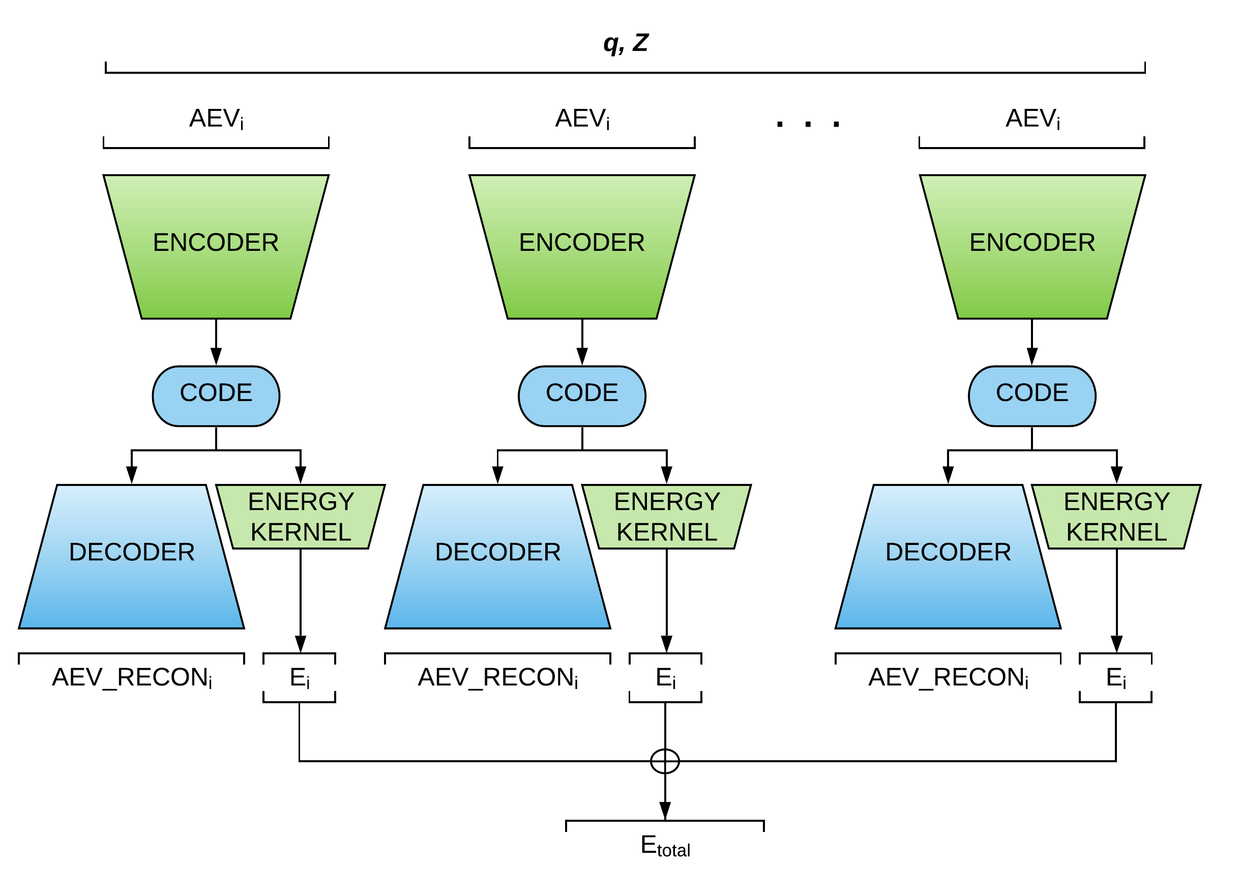Figure 3: ANIEncoder Architecture

The ANIEncoder architecture allows the incorporation of a vast amount of augmented data such as perturbed structures, low-level molecular dynamics trajectories, and noisy data. The network learns a smooth representation of multidimensional potential energy surface that will result in enhanced accuracy and generalization.

MTL Loss

On-the-fly balancing of all the loss terms is required to ensure equal emphasis for training all objectives in an MTL problem such as ANIEncoder. Otherwise, one task might dominate the overall loss and consecutively converge faster while others cannot reach their learning potential and are unable to affect the learning process of the shared layers in a given number of optimization iterations.

The naive approach is to consider the overall loss as the weighted linear sum of task-specific loss functions (\(L_{i}\)). The total loss requires \(N\) hyperparameters \(\omega_i\) for an \(N\)-task problem. 

\[L_{total}\ =\sum_i^{N}\omega_iL_i\]

However, the time and space complexity of finding the best set of hyperparameters using algorithms such as grid search substantially increases with the number of tasks in this case.

The task-specific prediction uncertainty can be employed to determine the relative confidence between different tasks (9, 10). The following mathematical formulation of this type of loss for MTL was introduced by Kendall et al. (9):

Let \(f\) be a neural network with parameters \(W\). Assuming Gaussian distribution for the underlying prediction error, the likelihood of prediction y is as follows:

\[p(y|f^{W}(x)) = \mathcal{N}(f^{W}(x), \sigma^{2})\]

The model can estimate both mean and variance \(\sigma^{2}\) (the observation noise) of output distribution given the input \(x\). In MTL problems where there exist multiple outputs of the model, the total likelihood becomes the multiplication of the task-specific probabilities. As an example for a two-task MTL:

\[p(y_1, y_2 | f^{W}(x)) = p(y_1 | f^{W}(x)) \cdot p(y_2 | f^{W}(x))\] \[= \mathcal{N}(y_1; f^{W}(x), \sigma_1^{2}) \cdot \mathcal{N}(y_2; f^{W}(x), \sigma_2^{2})\]

By performing maximum a posteriori estimation (MAP) inference, we can obtain an objective function to minimize:

\[-\log p(y_1, y_2 | f^{W}(x)) \propto \frac{1}{2\sigma_1^2} \||{y_1-f^{W}(x)}\||^{2} + \frac{1}{2\sigma_2^2} \||{y_2-f^{W}(x)}\||^{2} + \log \sigma_1 \sigma_2\] \[= \frac{1}{2\sigma_1^2} \mathcal{L}_1(W) + \frac{1}{2\sigma_2^2} \mathcal{L}_2(W) + \log \sigma_1 \sigma_2\]

Where \(\mathcal{L}_1\) and \(\mathcal{L}_2\) are the task-specific loss terms and can be replaced by squared error metrics often used as regression loss functions. Minimizing this MTL loss with respect to \(\sigma_{i}\) is equivalent to adaptively learning the relative weights of task-specific losses based on the data. The MTL loss was implemented for ANIEncoder to avoid using hyperparameters when training both energy learning and autoencoding tasks.

Results and discussion

ANIEncoder was trained on the ANI-1x dataset—a 5M DFT calculations of small organic molecules containing H, C, N, and O elements. The data were randomly split into %80/%20 training/validation. The network parameters for the autoencoding task were shared among all atomic networks and atomic energy kernels predict their contribution to the molecular energies using the representation learned in the unsupervised task. The evaluation results of ANIEncoder on COMP6 benchmark are provided in Table 1.

Model	Energy	Relative Energy	Forces
ANI-1x	1.93/3.37	1.85/2.95	3.09/5.29
ANIEncoder	2.17/3.35	2.19/3.37	3.98/6.29

Table 1: COMP6 benchmark (MAE/RMSE) results in kcal/mol (energies) and kcal/mol/A (forces)

The ANIEncoder MAE/RMSE metrics for the COMP6 dataset closely reproduce the ANI-1x model trained with the same dataset. However, hyperparameter tuning can help achieve identical or better performance. The training was found to be sensitive to the learning rate decay and the number of shared layers.

The MTL loss balances the learning pace of energy prediction and autoencoding tasks on the fly. However, data imbalance can bias the representation learning of different elements. The abundance of Hydrogens in our datasets biases the learning process. We can adjust the learning rate, the number of parameters, or regularizations applied to individual atomic energy kernels to account for the data imbalance. However, the representation learning task cannot distinguish the element types and therefore is biased towards Hydrogens.

Future work

ANIEncoder was trained on the ANI-1x dataset in which all the data points are labeled with their DFT energies. However, the advantage of this semi-supervised model is the ability to use unlabeled data, i.e., molecules without the QM energy labels. One way to achieve this is by adding random multivariate gaussian noise to the existing coordinates or perturbing the structure in the direction of the normal modes (normal mode sampling).

The amount of parameter sharing between different tasks can be adjusted depending on their similarity and constructiveness. We can decrease the amount of sharing if simultaneously learning multiple tasks is degrading the performance.

The experimental version of ANIEncoder will be publicly released after passing accuracy tests.

References

1. Aaronson, S. (2009). Why quantum chemistry is hard. Nature Physics, 5(10), 707-708.
2. Smith, J. S., Isayev, O., & Roitberg, A. E. (2017). ANI-1: an extensible neural network potential with DFT accuracy at force field computational cost. Chemical science, 8(4), 3192-3203.
3. Behler, J., & Parrinello, M. (2007). Generalized neural-network representation of high-dimensional potential-energy surfaces. Physical review letters, 98(14), 146401.
4. Gao, X., Ramezanghorbani, F., Isayev, O., Smith, J., & Roitberg, A. (2020). TorchANI: A Free and Open Source PyTorch Based Deep Learning Implementation of the ANI Neural Network Potentials. Journal of chemical information and modeling.
5. Smith, J. S., Nebgen, B., Lubbers, N., Isayev, O., & Roitberg, A. E. (2018). Less is more: Sampling chemical space with active learning. The Journal of chemical physics, 148(24), 241733.
6. Smith, J. S., Nebgen, B. T., Zubatyuk, R., Lubbers, N., Devereux, C., Barros, K., … & Roitberg, A. E. (2019). Approaching coupled cluster accuracy with a general-purpose neural network potential through transfer learning. Nature communications, 10(1), 1-8.
7. Devereux, C., Smith, J., Davis, K., Barros, K., Zubatyuk, R., Isayev, O., … & Isayev, O. (2020). Extending the applicability of the ANI deep learning molecular potential to Sulfur and Halogens. ChemRxiv.
8. Caruana, R. (1997). Multitask learning. Machine learning, 28(1), 41-75.
9. Kendall, A., Gal, Y., & Cipolla, R. (2018). Multi-task learning using uncertainty to weigh losses for scene geometry and semantics. In Proceedings of the IEEE conference on computer vision and pattern recognition (pp. 7482-7491).
10. Scalia, G., Grambow, C. A., Pernici, B., Li, Y. P., & Green, W. H. (2020). Evaluating Scalable Uncertainty Estimation Methods for Deep Learning-Based Molecular Property Prediction. Journal of Chemical Information and Modeling.

Acknowledgements

“Farhad Ramezanghorbani was supported by a fellowship from The Molecular Sciences Software Institute under NSF grant OAC-1547580”