
freud: Powerful, Efficient Trajectory Analysis in Scientific Python


![]()
Overview
The freud Python library provides a simple, flexible, powerful set of tools for analyzing trajectories obtained from molecular dynamics or Monte Carlo simulations. High performance, parallelized C++ is used to compute standard tools such as radial distribution functions, correlation functions, order parameters, and clusters, as well as original analysis methods including potentials of mean force and torque (PMFTs) and local environment matching. The freud library supports many input formats and outputs NumPy arrays, enabling integration with the scientific Python ecosystem for many typical materials science workflows.
The freud project released a new major version (2.0) in November 2019. This version brought new features including:
- A unified API for all analysis methods
- 4x performance improvements (on average) across a suite of common analysis methods
- Flexible neighbor-finding logic that can be used to accelerate user-defined analysis methods
- Trajectory reader integration, supporting 25+ file formats
- Cross-platform support for Linux, Mac, and Windows
Resources
- Reference Documentation: Examples, tutorials, topic guides, and package Python APIs.
- Installation Guide: Instructions for installing and compiling freud.
- freud-users Google Group: Ask questions to the freud user community.
- GitHub repository: Download the freud source code.
- Issue tracker: Report issues or request features.
Purpose of freud
Scope
The freud library is designed for analyzing colloidal and coarse-grained simulations, where particles are frequently mesoscopic in size and lack an “atomic identity” (see Figure 1). This makes freud suitable for applications in materials science, distinguishing the library from other packages that primary focus on biomolecular simulations such as MDAnalysis and MDTraj. Our recently published paper in Computer Physics Communications describes the features and design philosophy of freud [1]. A second paper in the Proceedings of the 18th Python in Science Conference (SciPy 2019) describes freud’s applications in machine learning and data visualization workflows in materials science, including integrations with the OVITO application and other visualization frameworks [2].
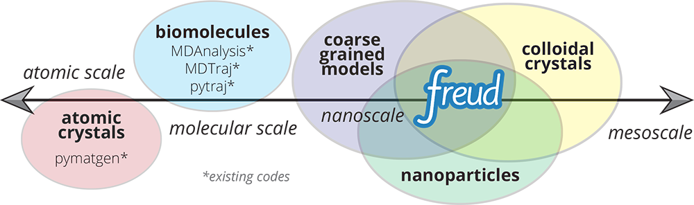 Figure 1: Common Python tools for simulation analysis at varying length scales. The freud library is designed for nanoscale systems, suchas colloidal crystals and nanoparticle assemblies. In such systems, interactions are described by coarse-grained models where particles’ atomic constituents are often irrelevant and particle anisotropy (non-spherical shape) is common, thus requiring a generalized concept of particle “types” and orientation-sensitive analyses. These features contrast the assumptions of most analysis tools designed for biomolecular simulations and materials science. Image and caption reproduced from [2] under a Creative Commons Attribution License.
Applications
The high performance, parallelized analysis methods in freud can be used to analyze systems of millions of particles [3] and perform real-time analysis for data visualization applications [2]. The freud library has been used to analyze kinetics of triblock Janus colloids, quantify evaporation-induced assembly, perform machine learning on crystal structures, optimize pair potentials, and more. A more extensive list of publications that have used freud can be found in our recent paper [1].
Core Data Structures
The core components of freud are described for users via the package documentation’s Tutorial. In short, all analyses in freud act on a “system,” which is composed of a periodic simulation box and an array of particle positions. The most common computation performed by the freud library is finding particles’ neighbors, which forms the core of almost all the analysis methods offered by the library. A visual depiction of how data flows through the freud library is shown in Figure 2.
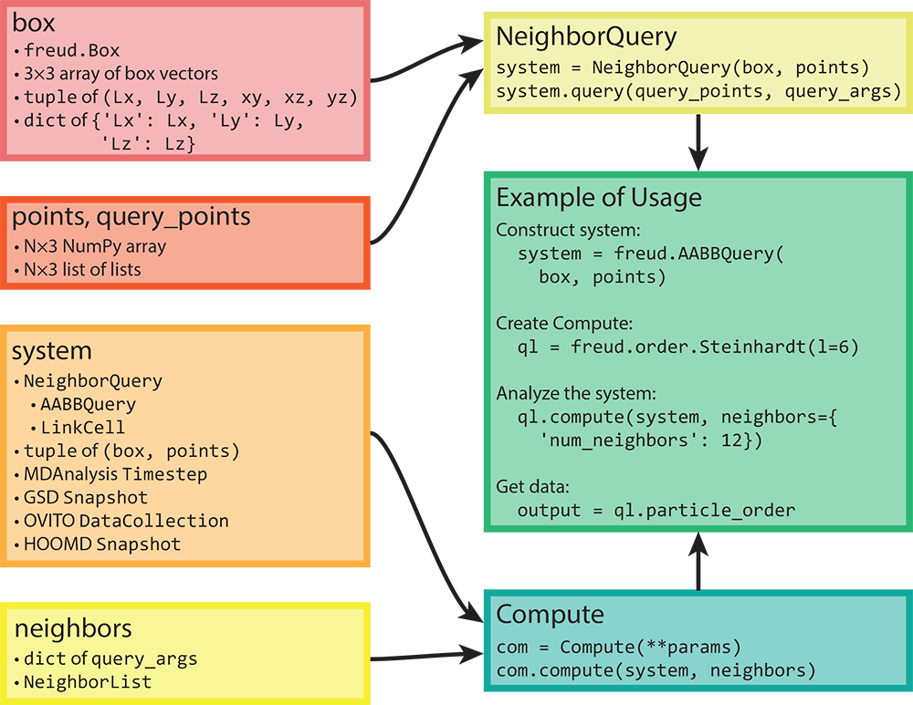 Figure 2: Here we show the flow of various types of inputs into freud. Boxes can be constructed based on a variety of inputs, all of which can also directly be provided anywhere a box object is required. Similarly, any object that can be interpreted as an array can be provided where particle positions are required. Any valid pair of box and points can be used to construct a
 NeighborQuery object, which is one of the types of systems that freud accepts. In addition to a NeighborQuery, freud can also interpret raw tuples of boxes and points as system objects, or use simulation frames from numerous external tools (a subset are shown in the figure). Any computation that involves finding nearest neighbors also requires a specification of neighbors, which can be a NeighborList or a dictionary of query arguments. The “Example of Usage” box on the right shows a typical use case of freud that combines these concepts. Reprinted from [1].
Analysis Methods
Standard Techniques
The freud library includes many analysis methods common to statistical mechanics and materials science, including the radial distribution function \(g(r)\), correlation functions (shown in Figure 3), and clustering algorithms. Additionally, the freud library incorporates the voro++ library for fast computations of Voronoi diagrams (shown in Figure 3). The library includes a wide range of order parameters useful for distinguishing phases and identifying crystal structures, including the Steinhardt order parameter and cubatic order parameter shown in Figure 4. All features, including code examples and sample figures, are shown in the freud documentation.
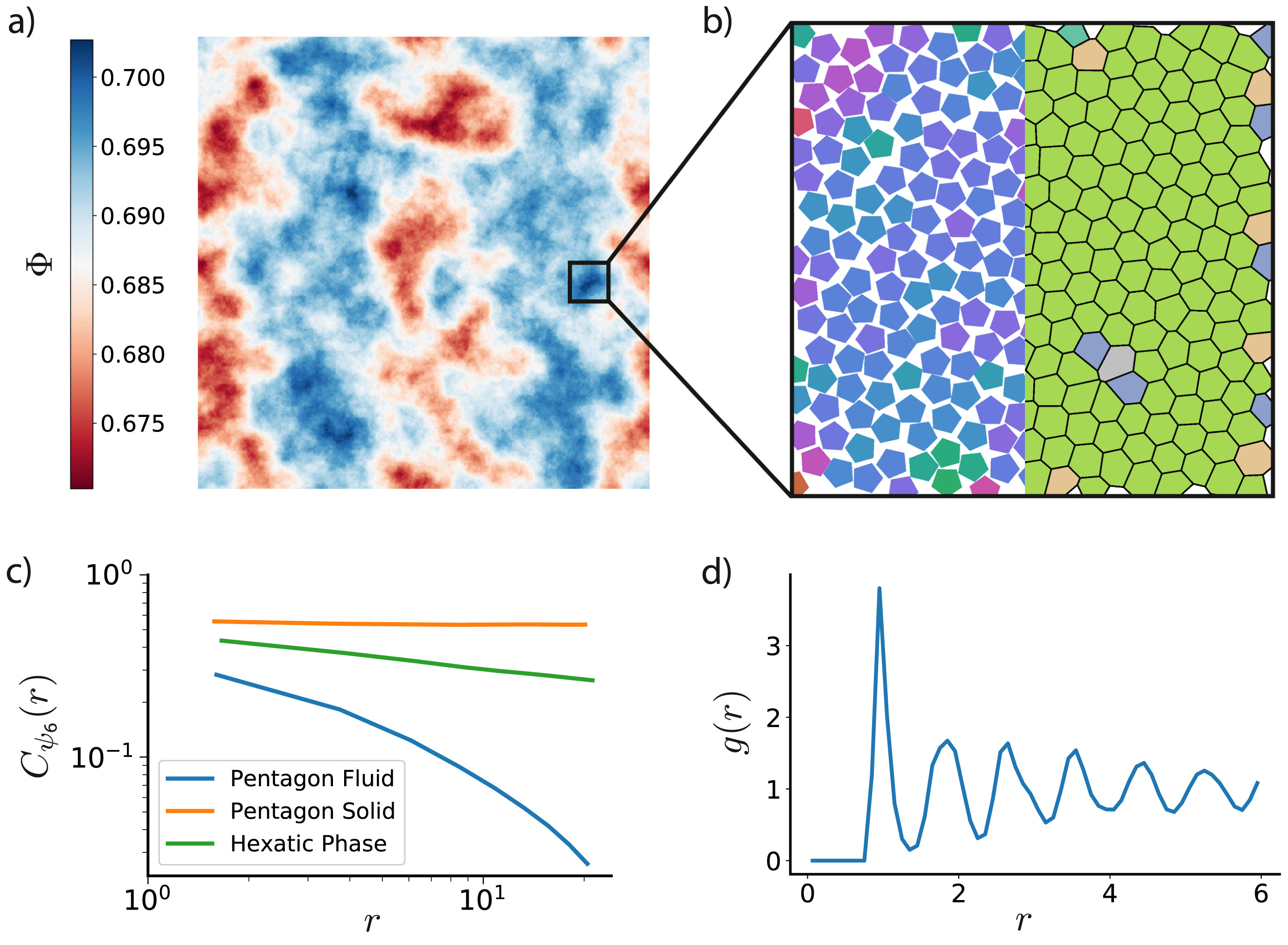 Figure 3: The freud library is capable of computing a number of characteristics of a system of particles. Here, we demonstrate some of those features on a 2D Monte Carlo simulation of polygons that exhibits hexatic ordering [3]. a) Phase separation is clearly evident in this system of pentagons colored by local density ; the system is divided into denser (blue) and less dense (red) regions. b) Zooming into a particularly dense region shows that the hexatic ordering (left half) is generally uniform across the region. The Voronoi diagram of the system (right half) is also largely defect-free, with just a few pentagons having more or fewer than 6 nearest neighbors. c) The spatial correlation of the hexatic order parameter is nearly constant for a nearly perfect crystal of pentagons (orange), whereas it decays very quickly in a fluid (blue). For a comparable system of hexagons, however, we see a power-law decay (green) in the hexatic order parameter due to the presence of a hexatic phase between the solid and fluid phases. d) The radial distribution function for the system of pentagons shows the expected sequence of neighbor shells as a function of distance. Reprinted from [1].
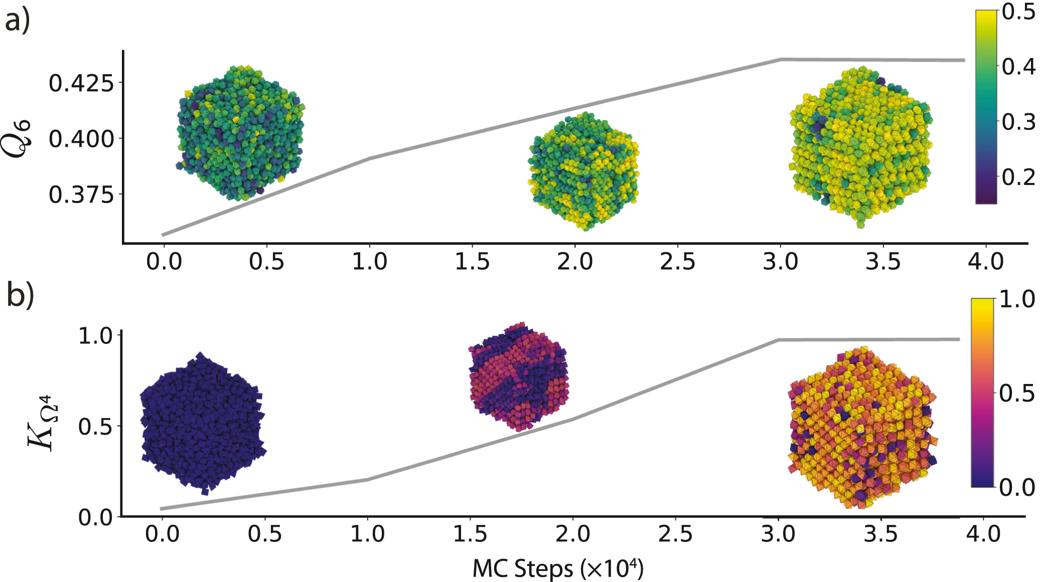 Figure 4: Various order parameters can be used to characterize the degree of ordering in a system. The per-particle order parameter values eventually converge to a uniform global value as the system becomes globally well-ordered. These plots show the evolution of two order parameters over the course of a Monte Carlo simulation of hard particles, which over time rearrange into an ordered phase under compression. Simulation snapshots are colored by the per-particle order parameter and rendered with fresnel. a) The Steinhardt \(Q_6\) order parameter is an appropriate scalar descriptor for systems forming a BCC (cI2-W) structure. Systems of cuboctahedra in the fluid phase show a distinctly different characteristic value of the order parameter than in the solid phase. b) The cubatic order parameter \(K_{\Omega^4}\) is useful for characterizing ordering in these systems of octahedra. Reprinted from [1].
Specialized Methods
Several analysis methods in freud are unique to the library and not implemented elsewhere.
Two modules with such unique features are pmft, which implements the Potential of Mean Force and Torque method shown in Figure 5, and environment, which contains several features for analyzing crystalline environments.
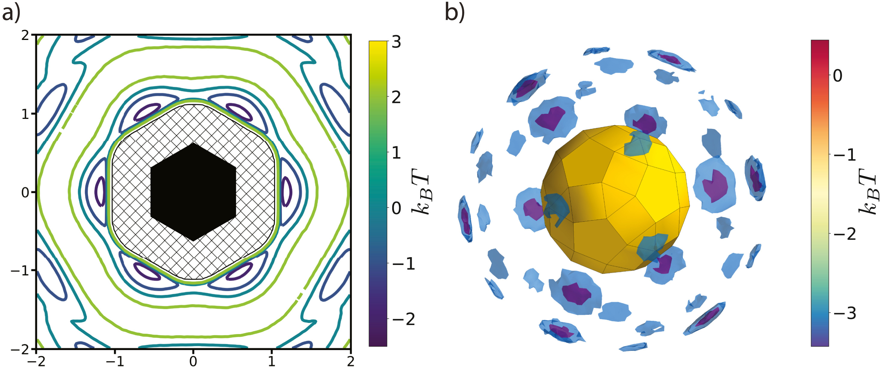 Figure 5: The PMFT is related to the probability of finding particles at a given position and orientation relative to one another. a) The PMFT of an ordered system of hexagons [4], where the locations of the wells indicate that particles are much more likely to sit next to the edges of their neighbors than the corners. In two-dimensional systems, the full PMFT is 3-dimensional, since it also must account for the orientation of the second particle relative to the first; for clarity, in this figure we have integrated out that degree of freedom. b) A PMFT computed from a system of rhombicosidodecahedra shows distributions of neighboring particles in three dimensions (figure rendered using Mayavi). There are six degrees of freedom in 3D systems, three translational and three rotational. This PMFT only shows the three translational degrees of freedom. The wells representing the deepest energy isosurfaces of the PMFT align with the largest (pentagonal) facets of the polyhedron. Reprinted from [1].
User-defined Analysis Methods
The core data structures for finding particle neighbors also enable user-defined analyses, where neighbor finding is handled by freud and user-defined code performs computations over the sets of neighbor bonds. For example, the example code below (an excerpt from a corresponding example in the documentation) implements Common Neighbor Analysis.
1
2
3
4
5
6
7
8
9
10
11
12
13
14
15
16

import freud
import numpy as np
from collections import defaultdict

# Use a face-centered cubic (fcc) system
box, points = freud.data.UnitCell.fcc().generate_system(4)
aq = freud.AABBQuery(box, points)
nl = aq.query(points, {'num_neighbors': 12, 'exclude_ii': True}).toNeighborList()

# Get all sets of common neighbors.
common_neighbors = defaultdict(list)
for i, p in enumerate(points):
    for j in nl.point_indices[nl.query_point_indices == i]:
        for k in nl.point_indices[nl.query_point_indices == j]:
            if i != k:
                common_neighbors[(i, k)].append(j)
Next, we use NetworkX to build graphs of common neighbors and compute the Common Neighbor Analysis signatures.
1
2
3
4
5
6
7
8
9
10
11
12
13
14
15
16
17
18
19
20
21
22
23
24
25
26
27
28
29
30
31
32
33
34
35
36
37
38

import networkx as nx
from collections import Counter

diagrams = defaultdict(list)
particle_counts = defaultdict(Counter)

for (a, b), neighbors in common_neighbors.items():
    # Build up the graph of connections between the
    # common neighbors of a and b.
    g = nx.Graph()
    for i in neighbors:
        for j in set(nl.point_indices[
            nl.query_point_indices == i]).intersection(neighbors):
            g.add_edge(i, j)

    # Define the identifiers for a CNA diagram:
    # The first integer is 1 if the particles are bonded, otherwise 2
    # The second integer is the number of shared neighbors
    # The third integer is the number of bonds among shared neighbors
    # The fourth integer is an index, just to ensure uniqueness of diagrams
    diagram_type = 2-int(b in nl.point_indices[nl.query_point_indices == a])
    key = (diagram_type, len(neighbors), g.number_of_edges())
    # If we've seen any neighborhood graphs with this signature,
    # we explicitly check if the two graphs are identical to
    # determine whether to save this one. Otherwise, we add
    # the new graph immediately.
    if key in diagrams:
        isomorphs = [nx.is_isomorphic(g, h) for h in diagrams[key]]
        if any(isomorphs):
            idx = isomorphs.index(True)
        else:
            diagrams[key].append(g)
            idx = diagrams[key].index(g)
    else:
        diagrams[key].append(g)
        idx = diagrams[key].index(g)
    cna_signature = key + (idx,)
    particle_counts[a].update([cna_signature])
Looking at the counts of common neighbor signatures, we see that the first particle of the fcc structure has 12 bonds with signature (1, 4, 2, 0) as we expect.
1

particle_counts[0]
Counter({(1, 4, 2, 0): 12,
         (2, 4, 4, 0): 6,
         (2, 1, 0, 0): 12,
         (2, 2, 1, 0): 24})
Open-Source Community
Integrations with the Scientific Python Ecosystem
Leveraging the NumPy library for data arrays allows freud to easily integrate with a wide variety of other packages in the scientific Python ecosystem.
Users of freud can execute analyses in a Jupyter notebook and use the plot() method of any compute object to see the results immediately without having to manually set axis labels or titles.
This plotting functionality uses Matplotlib, and can be used with user-provided Axis objects for additional customization.
The use of these standard scientific Python libraries, in addition to previously mentioned integrations with MDAnalysis, MDTraj, and OVITO, ensure freud is accessible to new users without significant alteration to their existing workflows.
User Support and External Contributions
The freud-users Google Group is available for user support, with responses typically within 1 business day. The freud library has had 39 code contributors, primarily from the University of Michigan, though several recent features have been developed in direct response to community requests from the Google Group or GitHub issue tracker. Whenever possible, the freud development team encourages pull requests and/or code review from external users in response to their feature requests or bug reports, building a shared sense of ownership in the results.
Impact of freud
Though it is extremely difficult to estimate the size of any package’s user base, metrics from the documentation web pages indicate that the number of freud users has grown significantly over the last two years. The package has been downloaded over 90,000 times from conda-forge and the number of users visiting freud’s documentation has grown substantially, shown in Figure 6.
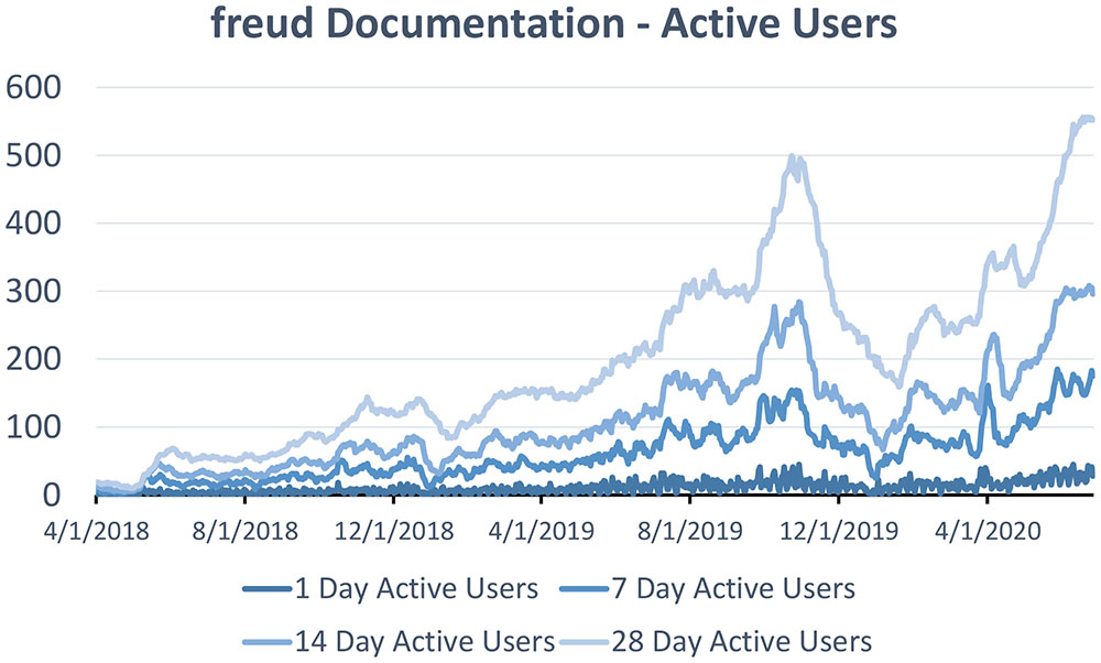 Figure 6: Daily active users visiting freud’s documentation in the last 1, 7, 14, or 28 days, from April 1, 2018 to June 26, 2020.
References
Figures 2, 3, 4, 5 are reprinted from [1], copyright 2020, with permission from Elsevier.
- V. Ramasubramani, B. D. Dice, E. S. Harper, M. P. Spellings, J. A. Anderson, and S. C. Glotzer. freud: A Software Suite for High Throughput Analysis of Particle Simulation Data. Computer Physics Communications Volume 254, September 2020, 107275. https://doi.org/10.1016/j.cpc.2020.107275.
- B. Dice, V. Ramasubramani, E. S. Harper, M. P. Spellings, J. A. Anderson, and S. C. Glotzer. Analyzing Particle Systems for Machine Learning and Data Visualization with freud. Proceedings of the 18th Python in Science Conf. (SciPy 2019), SciPy, 27-33. https://doi.org/10.25080/Majora-7ddc1dd1-004. See also this YouTube video of the freud talk at SciPy 2019.
- J. A. Anderson, J. Antonaglia, J. A. Millan, M. Engel, & S. C. Glotzer. Shape and Symmetry Determine Two-Dimensional Melting Transitions of Hard Regular Polygons. Physical Review X, 7(2), 021001 (2017). https://doi.org/10.1103/PhysRevX.7.021001.
- E. S. Harper, R. L. Marson, J. A. Anderson, G. van Anders, & S. C. Glotzer. Shape allophiles improve entropic assembly. Soft Matter, 11(37), 7250–7256 (2015). https://doi.org/10.1039/C5SM01351H.
Acknowledgements
Support for the design and development of freud has evolved over time and with programmatic research directions. A majority of the code development including all public code releases are supported by the National Science Foundation, Division of Materials Research under a Computational and Data-Enabled Science & Engineering Award # DMR 1409620 (2014-2018) and the Office of Advanced Cyberinfrastructure Award # OAC 1835612 (2018-2021). Conceptualization and early implementations were supported in part by the DOD/ASD (R&E) under Award No. N00244-09-1-0062 and also by the National Science Foundation, Integrative Graduate Education and Research Traineeship, Award # DGE 0903629 (E.S.H. and M.P.S.). Bradley Dice acknowledges fellowship support from the National Science Foundation under OAC-1547580, S212: Impl: The Molecular Sciences Software Institute and an earlier National Science Foundation Graduate Research Fellowship Grant # DGE 1256260 (2016-2019). Vyas Ramasubramani holds the 2019-2020 J. Robert Beyster Computational Innovation Graduate Fellowship at the University of Michigan. Computational resources and services supported in part by Advanced Research Computing at the University of Michigan, Ann Arbor. Any opinions, findings, and conclusions or recommendations expressed in this publication are those of the authors and do not necessarily reflect the views of the DOD/ASD (R&E).