Linear Fitting with statsmodels
Contents
Linear Fitting with statsmodels#
Overview
Questions:
How can I fit a linear equation using statsmodels?
How can I fit a linear equation with multiple variables using statsmodels?
Objectives:
Use statsmodels for linear regression.
In this module, we are going to use statsmodels to fit our linear model. We are going to use an interface which allows us to use dataframes and text formulas to specify the equations we want to fit. To import statsmodels, use import statsmodels.formula.api as smf.
First, we’ll use pandas to load the data we cleaned in session 2.
import os
import pandas as pd

import statsmodels.formula.api as smf
file_path = os.path.join("data", "potts_table1_clean.csv")
df = pd.read_csv(file_path)
df.info()
<class 'pandas.core.frame.DataFrame'>
RangeIndex: 37 entries, 0 to 36
Data columns (total 10 columns):
 #   Column     Non-Null Count  Dtype
---  ------     --------------  -----
 0   Compound   37 non-null     object
 1   log P      34 non-null     float64
 2   pi         37 non-null     float64
 3   Hd         37 non-null     float64
 4   Ha         37 non-null     float64
 5   MV         36 non-null     float64
 6   R_2        37 non-null     float64
 7   log K_oct  36 non-null     float64
 8   log K_hex  30 non-null     float64
 9   log K_hep  24 non-null     float64
dtypes: float64(9), object(1)
memory usage: 3.0+ KB
Next, we will use ordinary least squares (ols) to fit our equation. When you call ols, you give it a formula you would like to fit. The dependent variable goes on the left side, followed by a ~. Then you put the independent variables you want to fit. To fit log P as a function of MV, we would expect put log P ~ MV. However, since our dependent variable has a space in it, we must group it using a special syntax - Q('log P'). Finally, we fit the model using .fit().
regression = smf.ols("Q('log P') ~ MV", data=df).fit()
This performs a fit to your equation using ordinary least squares. You can get a summary of your model by calling .summary on the fit.
regression.summary()
| Dep. Variable: | Q('log P') | R-squared: | 0.446 |
|---|---|---|---|
| Model: | OLS | Adj. R-squared: | 0.428 |
| Method: | Least Squares | F-statistic: | 24.98 |
| Date: | Wed, 12 May 2021 | Prob (F-statistic): | 2.16e-05 |
| Time: | 13:54:47 | Log-Likelihood: | -34.474 |
| No. Observations: | 33 | AIC: | 72.95 |
| Df Residuals: | 31 | BIC: | 75.94 |
| Df Model: | 1 | ||
| Covariance Type: | nonrobust |
| coef | std err | t | P>|t| | [0.025 | 0.975] | |
|---|---|---|---|---|---|---|
| Intercept | -7.2469 | 0.362 | -20.002 | 0.000 | -7.986 | -6.508 |
| MV | 0.0271 | 0.005 | 4.998 | 0.000 | 0.016 | 0.038 |
| Omnibus: | 21.287 | Durbin-Watson: | 1.639 |
|---|---|---|---|
| Prob(Omnibus): | 0.000 | Jarque-Bera (JB): | 28.520 |
| Skew: | 1.802 | Prob(JB): | 6.41e-07 |
| Kurtosis: | 5.783 | Cond. No. | 196. |
Notes:
[1] Standard Errors assume that the covariance matrix of the errors is correctly specified.
regression.params
Intercept   -7.246871
MV           0.027056
dtype: float64
Fitted values are stored automatically in regression.fittedvalues.
regression.fittedvalues
0    -6.960075
1    -6.659752
2    -6.643518
3    -6.383779
4    -6.343195
5    -6.105100
6    -6.067222
7    -5.910296
9    -5.839950
10   -5.829127
11   -5.788543
13   -5.623500
14   -5.618089
15   -5.553154
16   -5.515276
17   -5.512570
18   -5.461163
19   -5.461163
20   -5.417873
22   -5.417873
23   -5.352939
24   -5.325882
25   -5.325882
27   -5.290709
28   -5.274476
29   -5.236597
30   -5.095905
31   -4.998503
32   -4.957918
33   -4.722530
34   -4.681945
35   -4.433029
36   -4.162467
dtype: float64
df["predicted_values"] = regression.fittedvalues
df.head()
| Compound | log P | pi | Hd | Ha | MV | R_2 | log K_oct | log K_hex | log K_hep | predicted_values | |
|---|---|---|---|---|---|---|---|---|---|---|---|
| 0 | water | -6.85 | 0.45 | 0.82 | 0.35 | 10.6 | 0.00 | -1.38 | NaN | NaN | -6.960075 |
| 1 | methanol | -6.68 | 0.44 | 0.43 | 0.47 | 21.7 | 0.28 | -0.73 | -2.42 | -2.80 | -6.659752 |
| 2 | methanoicacid | -7.08 | 0.60 | 0.75 | 0.38 | 22.3 | 0.30 | -0.54 | -3.93 | -3.63 | -6.643518 |
| 3 | ethanol | -6.66 | 0.42 | 0.37 | 0.48 | 31.9 | 0.25 | -0.32 | -2.24 | -2.10 | -6.383779 |
| 4 | ethanoicacid | -7.01 | 0.65 | 0.61 | 0.45 | 33.4 | 0.27 | -0.31 | -3.28 | -2.90 | -6.343195 |
You can make predictions using the fitted model by calling regression.predict and passing in values for which you want a prediction as part of a pandas dataframe with appropriate column names. Your column names must match the column names you performed the fit with.
help(regression.predict)
Help on method predict in module statsmodels.base.model:

predict(exog=None, transform=True, *args, **kwargs) method of statsmodels.regression.linear_model.OLSResults instance
    Call self.model.predict with self.params as the first argument.

    Parameters
    ----------
    exog : array_like, optional
        The values for which you want to predict. see Notes below.
    transform : bool, optional
        If the model was fit via a formula, do you want to pass
        exog through the formula. Default is True. E.g., if you fit
        a model y ~ log(x1) + log(x2), and transform is True, then
        you can pass a data structure that contains x1 and x2 in
        their original form. Otherwise, you'd need to log the data
        first.
    *args
        Additional arguments to pass to the model, see the
        predict method of the model for the details.
    **kwargs
        Additional keywords arguments to pass to the model, see the
        predict method of the model for the details.

    Returns
    -------
    array_like
        See self.model.predict.

    Notes
    -----
    The types of exog that are supported depends on whether a formula
    was used in the specification of the model.

    If a formula was used, then exog is processed in the same way as
    the original data. This transformation needs to have key access to the
    same variable names, and can be a pandas DataFrame or a dict like
    object that contains numpy arrays.

    If no formula was used, then the provided exog needs to have the
    same number of columns as the original exog in the model. No
    transformation of the data is performed except converting it to
    a numpy array.

    Row indices as in pandas data frames are supported, and added to the
    returned prediction.
to_predict = pd.DataFrame()
to_predict["MV"] = [75, 90]
regression.predict(to_predict)
0   -5.217658
1   -4.811815
dtype: float64
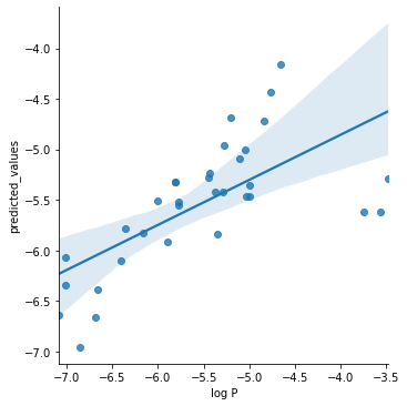
import seaborn as sns

g = sns.lmplot(x="log P", y="predicted_values", data=df)
Multiple Regression#
df.columns
Index(['Compound', 'log P', 'pi', 'Hd', 'Ha', 'MV', 'R_2', 'log K_oct',
       'log K_hex', 'log K_hep', 'predicted_values'],
      dtype='object')
multiple_regression = smf.ols("Q('log P') ~ pi + Hd + Ha + MV + R_2", data=df).fit()
multiple_regression.summary()
| Dep. Variable: | Q('log P') | R-squared: | 0.965 |
|---|---|---|---|
| Model: | OLS | Adj. R-squared: | 0.959 |
| Method: | Least Squares | F-statistic: | 150.4 |
| Date: | Wed, 12 May 2021 | Prob (F-statistic): | 7.87e-19 |
| Time: | 13:55:34 | Log-Likelihood: | 11.249 |
| No. Observations: | 33 | AIC: | -10.50 |
| Df Residuals: | 27 | BIC: | -1.518 |
| Df Model: | 5 | ||
| Covariance Type: | nonrobust |
| coef | std err | t | P>|t| | [0.025 | 0.975] | |
|---|---|---|---|---|---|---|
| Intercept | -4.4861 | 0.199 | -22.501 | 0.000 | -4.895 | -4.077 |
| pi | -0.9319 | 0.220 | -4.237 | 0.000 | -1.383 | -0.481 |
| Hd | -1.3037 | 0.185 | -7.038 | 0.000 | -1.684 | -0.924 |
| Ha | -4.3756 | 0.371 | -11.784 | 0.000 | -5.138 | -3.614 |
| MV | 0.0260 | 0.002 | 17.193 | 0.000 | 0.023 | 0.029 |
| R_2 | 0.5135 | 0.177 | 2.900 | 0.007 | 0.150 | 0.877 |
| Omnibus: | 0.688 | Durbin-Watson: | 1.300 |
|---|---|---|---|
| Prob(Omnibus): | 0.709 | Jarque-Bera (JB): | 0.200 |
| Skew: | 0.179 | Prob(JB): | 0.905 |
| Kurtosis: | 3.132 | Cond. No. | 835. |
Notes:
[1] Standard Errors assume that the covariance matrix of the errors is correctly specified.
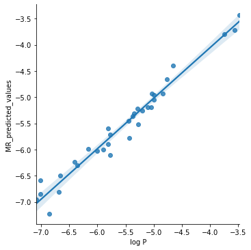
df["MR_predicted_values"] = multiple_regression.fittedvalues
g = sns.lmplot(x="log P", y="MR_predicted_values", data=df)
Key Points
Statsmodels allows you to specify your equations using data frames and column names.
Calling
.summary. on the fit gives you a summary of the fit and parameters.You can use
.predictto predict new values using the fitted model.You must give the predict method a dataframe with the same column names as the original dataframe.