OpenCAP: An open source package for studying resonances in molecules.

Motivation

Electronic states which are metastable with respect to electron detachment, known as resonances, play central roles in electron-molecule scattering processes occurring in various contexts, including chemistry, physics, and biology. Despite the ubiquity of these processes in nature, the computational infrastructure available to the scientific community for studying metastable electronic states lags far behind that available for treatment of bound electronic states. To help bridge this gap, we are developing OpenCAP, an open source software which extends the functionality of modern quantum chemistry packages to describe resonances.

Theory

Non-Hermitian Quantum Mechanics

Non-Hermitian quantum mechanics is a powerful tool for describing resonances that allows one to utilize quantum chemistry methodologies which have originally been developed for the study of bound electronic states. In non-Hermitian quantum mechanics formalisms, a resonance is associated with a single square-integrable state of a non-Hermitian Hamiltonian with a complex Siegert-Gamow energy. The real part of the energy \(E_{res}\) is the resonance position, and the imaginary part \(\Gamma\) is the half-width, which is inversely proportional to the lifetime of the state¹.

Complex Absorbing Potential (CAP)

The complex absorbing potential (CAP) is one of the few non-Hermitian formalisms which can be readily applied to molecules. In this approach, the electronic Hamiltonian is augmented with an artificial complex absorbing potential \(-i\eta W\), where \(\eta\) is the CAP strength parameter¹. The CAP absorbs the outgoing tail of the resonance wavefunction, transforming it into a square integrable eigenstate of the non-Hermitian Hamiltonian¹. When finite basis sets are used, \(E_{res}\) and \(\Gamma\) become \(\eta\) -dependent. The best estimate of resonance position and width is obtained by finding an optimal value \(\eta_{opt}\) which satisfies the minimum logarithmic velocity criteria¹.

\[min|\eta\frac{\mathrm{dE} }{\mathrm{d} \eta}|\]

\(\eta_{opt}\) is typically found by analyzing so called \(\eta\) -trajectories (see the last panel of Figure 1).

Here, we exploit a projected version of the CAP formalism², which treats the CAP as a first order perturbation in a basis of pre-computed eigenstates of a Hermitian Hamiltonian, yielding the following matrix equation:

\[H^{CAP} = H_0-i \eta W\]

Both \(H_0\) and \(W\) are computed once for a set of eigenstates, and the matrix elements of \(W\) are obtained using the one-electron reduced density matrices \(\rho^i\), and transition density matrices \(\gamma^{ij}\).

\[W_{ij}= \begin{Bmatrix} Tr\left[W^{AO}\gamma^{ij} \right ] ,& i \neq j \\ Tr\left[W^{AO}\rho^{i} \right ] ,& i=j \end{Bmatrix}\]

Eigenvalue trajectories can be analyzed at minimal additional computational effort by diagonalizing the reduced dimension \(H^{CAP}\) over a range of \(\eta\) values.

Workflow

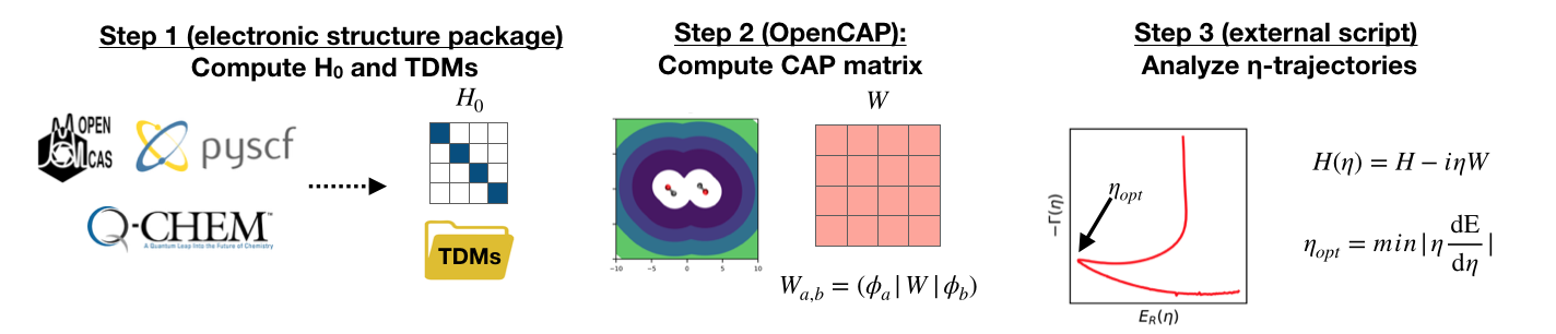
Figure 1: Workflow for conducting calculations with OpenCAP.

Step 1: Compute \(H_0\) and TDMs

The first step of any OpenCAP calculation is running an excited state electronic structure calculation with a supported package in order to generate the zeroth order Hamiltonian \(H_0\), and the set of one-electron reduced density and transition density matrices between each pair of eigenstates. These matrices can be read from disk (HDF5, formatted checkpoint) or passed directly in RAM when using the Python API.

Step 2: Compute CAP matrix

The CAP matrix is computed entirely by OpenCAP, first in atomic orbital basis, and then projected into the subspace of the real Hamiltonian using the one-electron reduced density and transition density matrices generated by the previous electronic structure calculation. To perform the projection of \(W\) into the subspace, the ordering of the basis functions of the CAP computed by OpenCAP must match the ordering of the density matrices computed by the electronic structure package.

Step 3: Analyze \(\eta\)-trajectories

Since the \(H_0\) and \(W\) matrices only need to be computed once, and can easily be stored, eigenvalue trajectories can be analyzed at the users convenience using a variety of analysis tools, such as Matplotlib or gnuplot.

Interfaces with Quantum Chemistry Packages

OpenCAP currently supports interfaces with the OpenMolcas³ and Pyscf⁴ packages, along with an interface to a locally modified version of Q-Chem⁵. OpenCAP supports two modes of operation: a standalone C++ executable, and a Python API.

Executable

When using the executable version of OpenCAP, the user prepares an input file as described in our documentation. Electronic structure data is read from disk, and OpenCAP prints the \(H_0\) and \(W\) matrices to standard output. The output can be analyzed using the script provided in our repository as a template. We have tested and obtained results using the executable version with OpenMolcas⁴ and a locally modified copy of Q-Chem.

opencap test.in > test.out
tail -23 test.out
Zeroth order Hamiltonian
-109.3052074400    0.0000000000   -0.0020964200    0.0000467200    0.0035367800   -0.0000949700    0.0020805500    0.0000616700   -0.0000000000    0.0000000000
   0.0000000000 -109.3052074400   -0.0000467200   -0.0020964000    0.0000949700    0.0035367800    0.0000616700   -0.0020805500    0.0000000000    0.0000000000
  -0.0020964200   -0.0000467200 -109.2407164400    0.0000000000    0.0270582400   -0.0001235400    0.0196302200    0.0001443500   -0.0000000000   -0.0000000000
   0.0000467200   -0.0020964000    0.0000000000 -109.2407160800    0.0001235400    0.0270583000    0.0001443500   -0.0196302500    0.0000000000    0.0000000000
   0.0035367800    0.0000949700    0.0270582400    0.0001235400 -109.2178091100    0.0000000000   -0.0482309000   -0.0001344500    0.0000000000    0.0000000000
  -0.0000949700    0.0035367800   -0.0001235400    0.0270583000    0.0000000000 -109.2178091100   -0.0001344500    0.0482309000    0.0000000000   -0.0000000000
   0.0020805500    0.0000616700    0.0196302200    0.0001443500   -0.0482309000   -0.0001344500 -109.0721414500   -0.0000000000   -0.0000000000    0.0000000000
   0.0000616700   -0.0020805500    0.0001443500   -0.0196302500   -0.0001344500    0.0482309000   -0.0000000000 -109.0721416100   -0.0000000000   -0.0000000000
  -0.0000000000    0.0000000000   -0.0000000000    0.0000000000    0.0000000000    0.0000000000   -0.0000000000   -0.0000000000 -109.0298915100    0.0000000000
   0.0000000000    0.0000000000   -0.0000000000    0.0000000000    0.0000000000   -0.0000000000    0.0000000000   -0.0000000000    0.0000000000 -109.0298916000
CAP matrix
-44.8078328210  -0.0000000000  21.8690451058  -0.4873519211  10.1088261447  -0.2714592872  -4.9300500373  -0.1461457678   0.0000000000  -0.0000000001
 -0.0000000000 -44.8078328201   0.4873519211  21.8690451052   0.2714592872  10.1088261454  -0.1461457678   4.9300500382  -0.0000000001  -0.0000000000
 21.8690451058   0.4873519211 -22.4698997766  -0.0000000000 -15.5224308448   0.0708743307  10.2163509455   0.0751310495  -0.0000000000   0.0000000003
 -0.4873519211  21.8690451052  -0.0000000000 -22.4698997752  -0.0708743307 -15.5224308447   0.0751310495 -10.2163509460   0.0000000003   0.0000000000
 10.1088261447   0.2714592872 -15.5224308448  -0.0708743307 -14.0795461907   0.0000000000  11.6779607539   0.0325580627  -0.0000000000   0.0000000004
 -0.2714592872  10.1088261454   0.0708743307 -15.5224308447   0.0000000000 -14.0795461911   0.0325580627 -11.6779607547   0.0000000004  -0.0000000000
 -4.9300500373  -0.1461457678  10.2163509455   0.0751310495  11.6779607539   0.0325580627 -11.5451058835   0.0000000000  -0.0000000001   0.0000000010
 -0.1461457678   4.9300500382   0.0751310495 -10.2163509460   0.0325580627 -11.6779607547   0.0000000000 -11.5451058846  -0.0000000010  -0.0000000000
  0.0000000000  -0.0000000001  -0.0000000000   0.0000000003  -0.0000000000   0.0000000004  -0.0000000001  -0.0000000010 -44.8627543309  -0.0000000000
 -0.0000000001  -0.0000000000   0.0000000003   0.0000000000   0.0000000004  -0.0000000000   0.0000000010  -0.0000000000  -0.0000000000 -44.8627543302
Wall time:2.4992220000

Python API

We currently have an experimental Python API which has been tested with OpenMolcas and Pyscf. Using the PyBind11 library, OpenCAP data structures and methods are exposed to Python, providing the user with direct control over the various parts of the calculation. After cloning the repository, OpenCAP can be installed as a python module called pycap.

import pycap
sys_dict = {"geometry":    '''N  0  0   1.039
                             N  0  0   -1.039
                            Gh 0  0   0.0''',
            "basis_file":"basis.bas",
            "bohr_coordinates": "true"}

cap_dict = {
            "cap_type": "box",
            "cap_x":"2.76",
            "cap_y":"2.76",
            "cap_z":"4.88",
            "Radial_precision": "14",
            "angular_points": "110"
}
nstates = 10 
package = "openmolcas"
# Defining classes
s = pycap.System(sys_dict)
pc = pycap.Projected_CAP(s,cap_dict,nstates,package)
... 
# Calling methods
pc.compute_ao_cap()
pc.compute_projected_cap()

Transition density matrices can be read from disk, or passed directly in RAM.

# Read data from disk
es_dict = {"method" : "ms-caspt2",
           "molcas_output":"anion_ms.out",
           "rassi_h5":"anion_ms.rassi.h5",
}
pc.read_data(es_dict)
mat=pc.get_projected_cap()
h0 = pc.get_H()

# pass TDM from state 1-->2 directly 
import h5py
import numpy as np
f = h5py.File('anion_ms.rassi.h5', 'r')
arr = f["SFS_TRANSITION_DENSITIES"]
arr1 = np.reshape(arr[0][1],(119,119))
pc.add_tdm(arr1,0,1)

Current Features

• Optimized numerical integration routines for computing the CAP matrix in atomic orbital basis
• Compatible with data generated by OpenMolcas, Pyscf, and Q-Chem
• Support for commonly used Box-type and Voronoi-type CAPs with user specified parameters
• Support for standard and custom ab initio basis sets specified in Psi4 format
• Easily modifiable sample scripts for eigenvalue trajectory analysis provided in the repository
• CMake cross platform build system

Application: \({}^2\Pi_g\) resonance of \(N_2^-\)

Our results for EOM-CCSD and CAP-XMS-CASPT2 are in agreement with previous theoretical and experimental results for this system, clearly demonstrating the potential of the OpenCAP approach for studying resonances. We note that our results for CAP-EOM-CCSD were obtained at a fraction of the computational cost as those reported by Zuev et al.⁶, as the original CAP-EOM-CCSD implementation in Q-Chem requires a unique electronic structure calculation for each \(\eta\) value.

\[\small \begin{array}{|c|c|c|c|} \hline \text{Method} & \text{Package} & E_{res} & \Gamma \\ \hline \text{CAP-EOM-CCSD}^6 & \text{QChem/Complex CCMAN2} & 2.48 & 0.42 \\ \hline \textbf{CAP-EOM-CCSD} & \text{QChem/OpenCAP} & 2.48 & 0.43 \\ \hline \text{CAP-XMCQDPT2}^7 & \text{Firefly} & 2.12 & 0.29 \\ \hline \textbf{CAP-XMS-CASPT2} & \text{OpenMolcas/OpenCAP} & 2.12 & 0.31 \\ \hline \text{Experiment}^8 & & 2.32 & 0.41 \\ \hline \end{array}\]

Conclusions

• OpenCAP is the first software of its kind which extends the functionality of modern quantum chemistry packages to describe resonances.
• The software functions as standalone executable and importable Python module.
• Our results obtained using supported interfaces show promising agreements with previous theoretical and experimental results.
• Future directions of the project include development of scattering-based approaches such as Feshbach Projection⁹ and R-matrix Theory¹⁰.

References

1. Riss, U. V.; Meyer, H. D. J. Phys. B At. Mol. Opt. Phys. 1993, 26 (23), 4503–4535.
2. Sommerfeld, T.; Santra, R. Int. J. Quantum Chem. 2001, 82 (5), 218–226.
3. Fdez. Galván, I.; Vacher, M.; Alavi, A.; Angeli, C.; Aquilante, F.; Autschbach, J.; Bao, J. J.; Bokarev, S. I.; Bogdanov, N. A.; Carlson, R. K.; et al. J. Chem. Theory Comput. 2019, 15 (11), 5925–5964.
4. Sun, Q.; Berkelbach, T. C.; Blunt, N. S.; Booth, G. H.; Guo, S.; Li, Z.; Liu, J.; McClain, J. D.; Sayfutyarova, E. R.; Sharma, S.; et al. WIREs Comput. Mol. Sci. 2018, 8 (1), e1340.
5. Shao, Y.; Gan, Z.; Epifanovsky, E.; Gilbert, A. T. B.; Wormit, M.; Kussmann, J.; Lange, A. W.; Behn, A.; Deng, J.; Feng, X.; et al. Mol. Phys. 2015, 113 (2), 184–215.
6. Zuev, D.; Jagau, T. C.; Bravaya, K. B.; Epifanovsky, E.; Shao, Y.; Sundstrom, E.; Head-Gordon, M.; Krylov, A. I. J. Chem. Phys. 2014, 141 (2).
7. Kunitsa, A. A.; Granovsky, A. A.; Bravaya, K. B. J. Chem. Phys. 2017, 146 (18).
8. M. Berman, H. Estrada, L. S. Cederbaum, and W. Domcke, Phys. Rev. A 28, 1363 (1983).
9. Feshbach, H. II. Ann. Phys. (N. Y). 1962, 19 (2), 287–313.
10. Tennyson, J. Phys. Rep. 2010, 491 (2), 29–76.

Acknowledgements

James Gayvert was supported by a fellowship from The Molecular Sciences Software Institute under NSF grant OAC-1547580.