Data Analysis using pandas#
Overview
Questions:
How do I analyze tabular data using Python?
What is pandas?
Objectives:
Use pandas to examine and analyze data.
Pandas is another Python package which is very popular for data analysis. The key data type of pandas is the dataframe. In this lesson, we will cover pandas dataframes and some basic analysis.
You are already familiar with the data analyis library numpy and the numpy array. NumPy is useful when you are working with data that is all numeric.
Pandas, however, is capable of handling data of lots of different types.
It is designed to make working with “relational” or “labeled” data easy and intuitive.
Central to the pandas package are the special data structures called pandas Series and DataFrames. Pandas dataframes are 2 dimensional and tabular, and is particularly suited to data which is heterogenous and in columns, like an SQL table or Excel spreadsheet. In fact, there are even functions which allow you to read data directly from excel spreadsheets or SQL databases.
Pandas is built to closely work with NumPy. Many functions which work on NumPy arrays will also work on Pandas DataFrames.
When pandas is imported, it is often shortened to pd.
In this notebook, we will be working with a data set that contains information about the elements in the periodic table.
The data is a csv (comma separated value) file from PubChem in your data folder called PubChemElements_all.csv.
This is a comma-separated value file, and we will use the pandas function read_csv. You can read more about this function in your Jupyter notebook by using
help(read_csv)
Library Documentation
Most popular Python libraries have very good online documentation.
You can find the pandas documentation by googling “pandas docs”.
You will be able to find the same help message you get for read_csv as well as tutorials and other types of documentation.
It is common to name the variable from the read_csv function df. This is short for DataFrame.
Since this file is relatively simple, we do not need any additional arguments to the function. The read_csv function reads in tabular data which is comma delimited by default.
import pandas as pd

df = pd.read_csv("data/PubChemElements_all.csv")
Examining the data#
The variable df is now a pandas DataFrame with the information contained in the csv file. You can examine the DataFrame using the .head() method.
This shows the first 5 rows stored in the DataFrame.
The first row of the file was used for column headers.
Functions vs Methods
In this lesson, we use the syntax variable.SOMETHING often.
When we do this, we are accessing special information or functions that act on variables. If the syntax is variable.SOMETHING(), with parenthesis it is a “method”, or function that acts on the variable. For example, if variable is a list, you might use the method variable.append(item) to add an item to the end of the list.
If it doesn’t have parenthesis, it is an “attribute” or data associated with the variable.
df.head()
| AtomicNumber | Symbol | Name | AtomicMass | CPKHexColor | ElectronConfiguration | Electronegativity | AtomicRadius | IonizationEnergy | ElectronAffinity | OxidationStates | StandardState | MeltingPoint | BoilingPoint | Density | GroupBlock | YearDiscovered | |
|---|---|---|---|---|---|---|---|---|---|---|---|---|---|---|---|---|---|
| 0 | 1 | H | Hydrogen | 1.008000 | FFFFFF | 1s1 | 2.20 | 120.0 | 13.598 | 0.754 | +1, -1 | Gas | 13.81 | 20.28 | 0.000090 | Nonmetal | 1766 |
| 1 | 2 | He | Helium | 4.002600 | D9FFFF | 1s2 | NaN | 140.0 | 24.587 | NaN | 0 | Gas | 0.95 | 4.22 | 0.000179 | Noble gas | 1868 |
| 2 | 3 | Li | Lithium | 7.000000 | CC80FF | [He]2s1 | 0.98 | 182.0 | 5.392 | 0.618 | +1 | Solid | 453.65 | 1615.00 | 0.534000 | Alkali metal | 1817 |
| 3 | 4 | Be | Beryllium | 9.012183 | C2FF00 | [He]2s2 | 1.57 | 153.0 | 9.323 | NaN | +2 | Solid | 1560.00 | 2744.00 | 1.850000 | Alkaline earth metal | 1798 |
| 4 | 5 | B | Boron | 10.810000 | FFB5B5 | [He]2s2 2p1 | 2.04 | 192.0 | 8.298 | 0.277 | +3 | Solid | 2348.00 | 4273.00 | 2.370000 | Metalloid | 1808 |
The .info function will give information about the columns and the data type of those columns. The data type will become very important later as we work with more data.
df.info()
<class 'pandas.core.frame.DataFrame'>
RangeIndex: 118 entries, 0 to 117
Data columns (total 17 columns):
 #   Column                 Non-Null Count  Dtype
---  ------                 --------------  -----
 0   AtomicNumber           118 non-null    int64
 1   Symbol                 118 non-null    object
 2   Name                   118 non-null    object
 3   AtomicMass             118 non-null    float64
 4   CPKHexColor            108 non-null    object
 5   ElectronConfiguration  118 non-null    object
 6   Electronegativity      95 non-null     float64
 7   AtomicRadius           99 non-null     float64
 8   IonizationEnergy       102 non-null    float64
 9   ElectronAffinity       57 non-null     float64
 10  OxidationStates        117 non-null    object
 11  StandardState          118 non-null    object
 12  MeltingPoint           103 non-null    float64
 13  BoilingPoint           93 non-null     float64
 14  Density                96 non-null     float64
 15  GroupBlock             118 non-null    object
 16  YearDiscovered         118 non-null    object
dtypes: float64(8), int64(1), object(8)
memory usage: 15.8+ KB
This output will show information about each column of data. Pandas assigns data types to columns, and will do its best to decide the data column for each column based on what is in the column. We can also see how many values are in each column.
We can also see descriptive statisics easily using the .describe() command.
df.describe()
| AtomicNumber | AtomicMass | Electronegativity | AtomicRadius | IonizationEnergy | ElectronAffinity | MeltingPoint | BoilingPoint | Density | |
|---|---|---|---|---|---|---|---|---|---|
| count | 118.000000 | 118.000000 | 95.000000 | 99.000000 | 102.000000 | 57.000000 | 103.000000 | 93.000000 | 96.000000 |
| mean | 59.500000 | 146.539858 | 1.732316 | 209.464646 | 7.997255 | 1.072140 | 1273.740553 | 2536.212473 | 7.608001 |
| std | 34.207699 | 89.768306 | 0.635187 | 38.569130 | 3.339066 | 0.879163 | 888.853859 | 1588.410919 | 5.878692 |
| min | 1.000000 | 1.008000 | 0.700000 | 120.000000 | 3.894000 | 0.079000 | 0.950000 | 4.220000 | 0.000090 |
| 25% | 30.250000 | 66.480750 | 1.290000 | 187.000000 | 6.020500 | 0.470000 | 516.040000 | 1180.000000 | 2.572500 |
| 50% | 59.500000 | 142.573830 | 1.620000 | 209.000000 | 6.960000 | 0.754000 | 1191.000000 | 2792.000000 | 7.072000 |
| 75% | 88.750000 | 226.777165 | 2.170000 | 232.000000 | 8.998500 | 1.350000 | 1806.500000 | 3618.000000 | 10.275250 |
| max | 118.000000 | 295.216000 | 3.980000 | 348.000000 | 24.587000 | 3.617000 | 3823.000000 | 5869.000000 | 22.570000 |
The describe function lists the mean, max, min, standard deviation and percentiles for each column excluding NaN (not a number) values.
Accessing Data in DataFrames#
One way to get information in a data frame is by using the headers, or the column names using squre brackets. The synatx for this is
dataframe["column_name"]
For example, to get the column with information about the atomic symbol, we would use the “Symbol” column.
df["Symbol"]
0       H
1      He
2      Li
3      Be
4       B
       ..
113    Fl
114    Mc
115    Lv
116    Ts
117    Og
Name: Symbol, Length: 118, dtype: object
If you want to select multiple columns, you use a list of column names in square brackets.
df[["Symbol", "AtomicNumber"]]
| Symbol | AtomicNumber | |
|---|---|---|
| 0 | H | 1 |
| 1 | He | 2 |
| 2 | Li | 3 |
| 3 | Be | 4 |
| 4 | B | 5 |
| ... | ... | ... |
| 113 | Fl | 114 |
| 114 | Mc | 115 |
| 115 | Lv | 116 |
| 116 | Ts | 117 |
| 117 | Og | 118 |
118 rows × 2 columns
If we want to get information in the dataframe using row and column numbers, we use the iloc function.
The syntax for iloc is
dataframe.iloc[row_number, column_number]
If you specify only a row number, you will get all the columns.
# This will get the first row, all of the columns.
df.iloc[0]
AtomicNumber                    1
Symbol                          H
Name                     Hydrogen
AtomicMass                  1.008
CPKHexColor                FFFFFF
ElectronConfiguration         1s1
Electronegativity             2.2
AtomicRadius                120.0
IonizationEnergy           13.598
ElectronAffinity            0.754
OxidationStates            +1, -1
StandardState                 Gas
MeltingPoint                13.81
BoilingPoint                20.28
Density                   0.00009
GroupBlock               Nonmetal
YearDiscovered               1766
Name: 0, dtype: object
# This will get the first row and the second column.
df.iloc[0, 1]
'H'
Performing Calculations#
Like NumPy arrays, pandas dataframes have features that let you avoid for loops.
For example, if you wanted to calculate the melting point of each
elemnt in celsius, you could do
df["MeltingPoint"] - 273.15
0      -259.34
1      -272.20
2       180.50
3      1286.85
4      2074.85
        ...
113        NaN
114        NaN
115        NaN
116        NaN
117        NaN
Name: MeltingPoint, Length: 118, dtype: float64
To save your calculation in a new column in your dataframe, use the syntax
df["new_column_name"] = CALCULATION
df["MeltingPointC"] = df["MeltingPoint"] - 273.15
If you have a more complicated action you’d like to peform for every column, you can use the syntax
df["column_name"].apply(FUNCTION)
where FUNCTION is a function that exists (like len) or a function that you’ve defined.
Consider a function to calculate the temperature in Farhenheit from Celsius.
def kelvin_to_fahrenheit(kelvin_temp):
    fahrenheit = (kelvin_temp - 273.15) * 9/5 +32
    return fahrenheit
If you wanted to apply this function to every row, your first instinct might be to write a for loop. This would work, but pandas has a built in method called apply to easily allow you to do this.
When you call the apply method, you give it a function name which you would like to apply to every element of whatever you are using it on.
# Calculate the boiling point in fahrenheit
df['BoilingPoint'].apply(kelvin_to_fahrenheit)
0      -423.166
1      -452.074
2      2447.330
3      4479.530
4      7231.730
         ...
113         NaN
114         NaN
115         NaN
116         NaN
117         NaN
Name: BoilingPoint, Length: 118, dtype: float64
Saving a new DataFrame#
If you wanted to save your data to a csv, you could do it using the method to_csv.
df.to_csv('periodic_data_processed.csv')
Filtering Data#
df["BoilingPoint"] > 300
0      False
1      False
2       True
3       True
4       True
       ...
113    False
114    False
115    False
116    False
117    False
Name: BoilingPoint, Length: 118, dtype: bool
Grouping Data#
You can perform operations like grouping data by category using pands. For this analysis, we will group elements by their standard state.
grouped_data = df.groupby(by="StandardState")
This is now essentially a group of dataframes.
If we use describe, we will get separate statistics for each group.
grouped_data.describe()
| AtomicNumber | AtomicMass | ... | Density | MeltingPointC | |||||||||||||||||
|---|---|---|---|---|---|---|---|---|---|---|---|---|---|---|---|---|---|---|---|---|---|
| count | mean | std | min | 25% | 50% | 75% | max | count | mean | ... | 75% | max | count | mean | std | min | 25% | 50% | 75% | max | |
| StandardState | |||||||||||||||||||||
| Expected to be a Gas | 1.0 | 118.000000 | NaN | 118.0 | 118.00 | 118.0 | 118.00 | 118.0 | 1.0 | 295.216000 | ... | NaN | NaN | 0.0 | NaN | NaN | NaN | NaN | NaN | NaN | NaN |
| Expected to be a Solid | 8.0 | 113.500000 | 2.449490 | 110.0 | 111.75 | 113.5 | 115.25 | 117.0 | 8.0 | 288.062500 | ... | NaN | NaN | 0.0 | NaN | NaN | NaN | NaN | NaN | NaN | NaN |
| Gas | 11.0 | 22.545455 | 26.322476 | 1.0 | 7.50 | 10.0 | 27.00 | 86.0 | 11.0 | 53.332053 | ... | 0.003474 | 0.00973 | 11.0 | -187.244545 | 67.941536 | -272.20 | -234.1050 | -210.000 | -134.5750 | -71.15 |
| Liquid | 2.0 | 57.500000 | 31.819805 | 35.0 | 46.25 | 57.5 | 68.75 | 80.0 | 2.0 | 140.245000 | ... | 10.927700 | 13.53360 | 2.0 | -23.015000 | 22.365787 | -38.83 | -30.9225 | -23.015 | -15.1075 | -7.20 |
| Solid | 96.0 | 58.666667 | 30.275808 | 3.0 | 32.75 | 59.5 | 84.25 | 109.0 | 96.0 | 144.008799 | ... | 11.171000 | 22.57000 | 90.0 | 1168.517189 | 823.705160 | 26.85 | 640.8500 | 1050.350 | 1552.3875 | 3549.85 |
5 rows × 80 columns
Similarly, we can see statistics for each group when using a method like .mean().
grouped_data["BoilingPoint"].mean()
StandardState
Expected to be a Gas              NaN
Expected to be a Solid            NaN
Gas                        102.452727
Liquid                     480.915000
Solid                     2922.236875
Name: BoilingPoint, dtype: float64
Built-In Plotting#
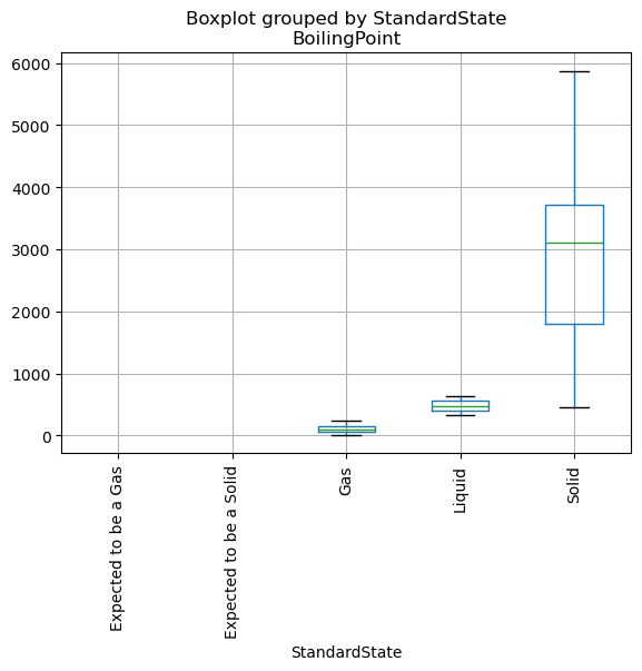
Pandas has numerous options for built-in plotting. We will only show a simple example here.
df.boxplot(column="BoilingPoint", by="StandardState", rot=90)
<Axes: title={'center': 'BoilingPoint'}, xlabel='StandardState'>